Reject Inference
N.B.: ce post s’inspire librement de mon manuscrit de thèse.
The granting process of all credit institutions is based on the probability that the applicant will refund his loan given his characteristics. This probability also called score is learnt based on a dataset in which rejected applicants are de facto excluded. This implies that the population on which the score is used will be different from the learning population. Thus, this biased learning can have consequences on the scorecard’s relevance. Many methods dubbed “reject inference” have been developed in order to try to exploit the data available from the rejected applicants to build the score. However most of these methods are considered from an empirical point of view, and there is some lack of formalization of the assumptions that are really made, and of the theoretical properties that can be expected. We propose a formalisation of these usually hidden assumptions for some of the most common reject inference methods, and we discus the improvement that can be expected. These conclusions are illustrated on simulated data and on real data from CACF.
Introduction
In consumer loans, the acceptance process can be formalized as follows. For a new applicant’s profile and credit’s characteristics, the lender aims at estimating the repayment probability. To this end, the credit modeler fits a predictive model, often a logistic regression, between already financed clients’ characteristics \(\boldsymbol{x}=(x_1,\ldots,x_d)\) and their repayment status, a binary variable \(y\in\{0,1\}\) (where 1 corresponds to good clients and 0 to bad clients). The model is then applied to the new applicant and yields an estimate of its repayment probability, called score after an increasing transformation. Under some cut-off value of the score, the applicant is rejected, except if further expert rules come into play as can be seen from Figure [1].
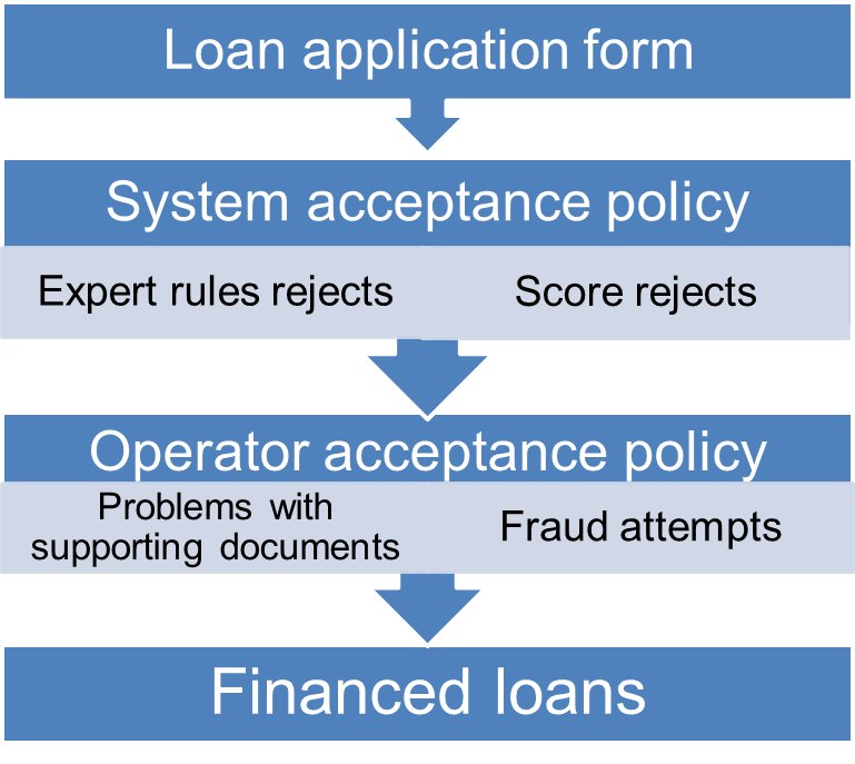
The through-the-door population (all applicants) can be classified into two categories thanks to a binary variable z taking values in \(\{\text{f},\text{nf}\}\) where \(\text{f}\) stands for financed applicants and \(\text{nf}\) for not financed ones. As the repayment variable \(y\) is unobserved for not financed applicants, credit scorecards are only constructed on financed clients’ data but then applied to the whole through-the-door population. The relevance of this process is a natural question which is dealt in the field of reject inference. The idea is to use the characteristics of not financed clients in the scorecard building process to avoid a population bias, and thus to improve the prediction on the whole through-the-door population. Such methods have been described in [36], [46], [43], [47], and have also notably been investigated in [44] who first saw reject inference as a missing data problem. In [39], the misspecified model case on real data is studied specifically and is also developed here.
In fact, it can be considered as a part of the semi-supervised learning setting, which consists in learning from both labelled and unlabelled data. However, in the semi-supervised setting [8] it is generally assumed that labelled data and unlabelled data come from the same distribution, which is rarely the case in Credit Scoring. Moreover, the main use case of semi-supervised learning is when the number of unlabelled data is far larger than the number of labelled data, which is not the case in Credit Scoring since the number of rejected clients and accepted clients is often balanced and depends heavily on the financial institution, the portfolio considered, etc.
The purpose of the present post is twofold: a clarification of which mathematical hypotheses, if any, underlie those reject inference methods and a clear conclusion on their relevance. In Section 1.2, we present a criterion to assess a method’s performance and discuss missingness mechanisms that characterize the relationship of \(z\) with respect to \(\boldsymbol{x}\) and \(y\). In Section 1.3, we go through some of the most common reject inference methods and exhibit their mathematical properties. To confirm our theoretical findings, we test each method on real data from Crédit Agricole Consumer Finance in Section 1.4. Finally, some guidelines are given to practitioners in Section 1.5.
Credit Scoring modelling
Data
The decision process of financial institutions to accept a credit application is usually embedded in the probabilistic framework. The latter offers rigorous tools for taking into account both the variability of applicants and the uncertainty on their ability to pay back the loan. In this context, the important term is \(p(y|\boldsymbol{x})\), designing the probability that a new applicant (described by his characteristics \(\boldsymbol{x}\)) will pay back his loan (\(y=1\)) or not (\(y=0\)). Estimation of \(p(y|\boldsymbol{x})\) is thus an essential task of any Credit Scoring process.
To perform estimation, a specific n + n'-sample \(\mathcal{T}\) is available, decomposed into two disjoint and meaningful subsets, denoted by \(\mathcal{T}_{\text{f}}\) and \(\mathcal{T}_{\text{nf}}\) (\(\mathcal{T}=\mathcal{T}_{\text{f}} \cup \mathcal{T}_{\text{nf}}\), \(\mathcal{T}_{\text{f}} \cap \mathcal{T}_{\text{nf}}=\emptyset\)). The first subset (\(\mathcal{T}_{\text{f}}\)) corresponds to n applicants with features \(\boldsymbol{x}_i\) who have been financed (\(z_i={\text{f}}\)) and, consequently, for who the repayment status \(y_i\) is known, with their respective matrix notation \(\boldsymbol{\mathbf{x}}_\text{f}\), \(\boldsymbol{\mathbf{z}}_\text{f}\) and \(\boldsymbol{\mathbf{y}}_\text{f}\). Thus, \(\mathcal{T}_{\text{f}}=(\boldsymbol{x}_i,y_i,z_i)_{i\in \text{F}} = (\boldsymbol{\mathbf{x}}_\text{f},\boldsymbol{\mathbf{y}}_\text{f},\boldsymbol{\mathbf{z}}_\text{f})\) where \(\text{F}=\{i:z_i={\text{f}}\}\) denotes the corresponding subset of indexes. The second subset (\(\mathcal{T}_{\text{nf}}\)) corresponds to n′ applicants with features \(\boldsymbol{x}_i\) who have not been financed (\(z_i={\text{nf}}\)) and, consequently, for who the repayment status \(y_i\) is unknown, with their respective matrix notation \(\boldsymbol{\mathbf{x}}_{\text{nf}}\) and \(\boldsymbol{\mathbf{z}}_{\text{nf}}\). Thus, \(\mathcal{T}_{\text{nf}}=(\boldsymbol{x}_i,z_i)_{i\in \text{NF}} = (\boldsymbol{\mathbf{x}}_{\text{nf}}, \boldsymbol{\mathbf{z}}_{\text{nf}})\) where \(\text{NF}=\{i:z_i={\text{nf}}\}\) denotes the corresponding subset of indexes. We notice that \(y_i\) values are excluded from the observed sample \(\mathcal{T}_{\text{nf}}\), since they are missing. These data can be represented schematically as:
$$\mathcal{T} = \begin{array}{c}
\mathcal{T}_{\text{f}} = \bigg( \; \boldsymbol{\mathbf{x}}_{\text{f}} \\
\\
\cup \\
\\
\mathcal{T}_{\text{nf}} = \bigg( \; \boldsymbol{\mathbf{x}}_{\text{nf}} \end{array}
\left( \begin{array}{ccc}
%\rowcolor{red!20}
\; \; x_{1,1} & \cdots & x_{1,d} \\
\vdots & \vdots & \vdots \\
x_{n,1} & \cdots & x_{n,d} \\
\; \; x_{n+1,1} & \cdots & x_{n+1,d} \\
\vdots & \vdots & \vdots \\
x_{n+n',1} & \cdots & x_{n+n',d} \end{array} \right),
\hspace{1.5cm}
\begin{array}{c}
\boldsymbol{\mathbf{y}}_{\text{f}} \\
\\
\\
\\
\boldsymbol{\mathbf{y}}_{\text{nf}} \end{array}
\left( \begin{array}{c}
y_1 \\
\vdots \\
y_n \\
\text{NA} \\
\vdots \\
\text{NA} \end{array} \right) ,
\hspace{1.5cm}
\begin{array}{c}
\boldsymbol{\mathbf{z}}_{\text{f}} \\
\\
\\
\\
\boldsymbol{\mathbf{z}}_{\text{nf}} \end{array}
\left( \begin{array}{c}
\text{f} \\
\vdots \\
\text{f} \\
\text{nf} \\
\vdots \\
\text{nf} \end{array} \right)
\hspace{0.2cm}
\begin{array}{c}
\bigg). \\
\\
\\
\\
\bigg). \end{array}$$
General parametric model
Estimation of \(p(y|\boldsymbol{x})\) has to rely on modelling since the true probability distribution is unknown. Firstly, it is both convenient and realistic to assume that triplets in \(\mathcal{T}_{\text{c}} = (\boldsymbol{x}_i,y_i,z_i)_{1\le i\le n+n'}\) are all independent and identically distributed (i.i.d.), including the unknown values of \(y_i\) when \(i\in \text{NF}\). Secondly, it is usual and convenient to assume that the unknown distribution \(p(y|\boldsymbol{x})\) belongs to a given parametric family \(\{p_{\boldsymbol{\theta}}(y|\boldsymbol{x})\}_{\boldsymbol{\theta} \in\Theta}\), where Θ is the parameter space. For instance, logistic regression is often considered in practice, even if we will be more general in this section. However, logistic regression will be important for other sections since some standard reject inference methods are specific to this family (Section 1.3) and numerical experiments (Section 1.4) will implement them.
As in any missing data situation (here \(z\) indicates if \(y\) is observed or not), the relative modelling process, namely \(p(z|\boldsymbol{x},y)\), has also to be clarified. For convenience, we can also consider a parametric family \(\{p_{\boldsymbol{\phi}}(z|\boldsymbol{x},y)\}_{\boldsymbol{\phi} \in \Phi}\), where \(\boldsymbol{\phi}\) denotes the parameter and Φ the associated parameter space of the financing mechanism. Note we consider here the most general missing data situation, namely a mechanism [23]. It means that \(z\) can be stochastically dependent on some missing data \(y\), namely that \(p(z|\boldsymbol{x},y)\neq p(z|\boldsymbol{x})\). We will discuss this fact in Section 1.2.4.
Finally, combining both previous distributions \(p_{\boldsymbol{\theta}}(y|\boldsymbol{x})\) and \(p_{\boldsymbol{\phi}}(z|\boldsymbol{x},y)\) leads to express the joint distribution of \((y,z)\) conditionally to \(\boldsymbol{x}\) as:
$$\label{eq:generative}
p_{\gamma}(y,z|\boldsymbol{x}) = p_{\boldsymbol{\phi}(\gamma)}(z|y,\boldsymbol{x})p_{\boldsymbol{\theta}(\gamma)}(y|\boldsymbol{x})$$
where \(\{p_{\gamma}(y,z|\boldsymbol{x})\}_{\gamma \in \Gamma}\) denotes a distribution family indexed by a parameter γ evolving in a space Γ. Here it is clearly expressed that both parameters \(\boldsymbol{\phi}\) and \(\boldsymbol{\theta}\) can depend on γ, even if in the following we will note shortly \(\boldsymbol{\phi}=\boldsymbol{\phi}(\gamma)\) and \(\boldsymbol{\theta}=\boldsymbol{\theta}(\gamma)\). In this very general missing data situation, the missing process is said to be non-ignorable, meaning that parameters \(\boldsymbol{\phi}\) and \(\boldsymbol{\theta}\) can be functionally dependent (thus \(\gamma\neq (\boldsymbol{\phi},\boldsymbol{\theta})\)). We also discuss this fact in Section 1.2.4.
Maximum likelihood estimation
Mixing previous model and data, the maximum likelihood principle can be invoked for estimating the whole parameter γ, thus yielding as a by-product an estimate of the parameter \(\boldsymbol{\theta}\). Indeed, \(\boldsymbol{\theta}\) is of particular interest, the goal of the financial institutions being solely to obtain an estimate of \(p_{\boldsymbol{\theta}}(y|\boldsymbol{x})\). The observed log-likelihood can be written as:
$$\label{eq:like.MNAR}
\ell(\gamma;\mathcal{T}) = \sum_{i\in\text{F}}\ln p_{\gamma}(y_i,\text{f} | \boldsymbol{x}_i) + \sum_{i'\in\text{NF}} \ln \left[ \sum_{y\in\{0,1\}} p_{\gamma}(y,\text{nf} | \boldsymbol{x}_{i'}) \right].$$
Within this missing data paradigm, the EM algorithm (see [14]) can be used: it aims at maximizing the expectation of the complete likelihood ℓc(γ; \(\mathcal{T}_c\) (defined hereafter) where \(\mathcal{T}_{\text{c}} = \mathcal{T} \cup \boldsymbol{\mathbf{y}}_{\text{nf}}\) over the missing labels. Starting from an initial value γ(0), iteration (s) of the algorithm is decomposed into the following two classical steps:
E-step
compute the conditional probabilities of missing \(y_i\) values:
$$t_{iy}^{(s)} = p_{\boldsymbol{\theta}(\gamma^{(s-1)})}(y|\boldsymbol{x}_i,\text{nf}) = \frac{p_{\gamma^{(s-1)}}(y, \text{nf}|\boldsymbol{x}_i)}{\sum_{y' = 0}^{1} p_{\gamma^{(s-1)}}(y', \text{nf}|\boldsymbol{x}_i)};$$
M-step
maximize the conditional expectation of the complete log-likelihood:
$$\label{eq:like.c}
\ell_c(\gamma;\mathcal{T}_{\text{c}}) = \sum_{i=1}^{n+n'}\ln p_{\gamma}(y_i,z_i | \boldsymbol{x}_i) = \sum_{i=1}^{n}\ln p_{\gamma}(y_i,\text{f} | \boldsymbol{x}_i) + \sum_{i=n+1}^{n+n'}\ln p_{\gamma}(y_i,\text{nf} | \boldsymbol{x}_i);$$
leading to:
$$\begin{aligned}
\gamma^{(s)} & = \arg\max_{\gamma \in \Gamma} \mathbb{E}_{\boldsymbol{\mathbf{y}}_{\text{nf}}} [\ell_c(\gamma;\mathcal{T}_{\text{c}}) | \mathcal{T},\gamma^{(s-1)}] \\
& = \arg\max_{\gamma \in \Gamma} \sum_{i\in \text{F}} \ln p_{\gamma}(y_i, \text{f}|\boldsymbol{x}_i) + \sum_{i'\in \text{NF}}\sum_{y = 0}^{1}t_{i'y}^{(s)} \ln p_{\gamma}(y, \text{nf} | \boldsymbol{x}_{i'}).\end{aligned}$$
Usually, stopping rules rely either on a predefined number of iterations, or on a predefined stability criterion of the observed log-likelihood.
Some current restrictive missingness mechanisms
The latter parametric family is very general since it considers both that the missingness mechanism is MNAR and non-ignorable. But in practice, it is common to consider ignorable models for the sake of simplicity, meaning that \(\gamma= (\boldsymbol{\phi},\boldsymbol{\theta})\). There exists also some restrictions to the MNAR mechanism.
The first restriction to MNAR is the MCAR setting, meaning that \(p(z| \boldsymbol{x},y) = p(z)\). In that case, applicants should be accepted or rejected without taking into account their descriptors \(\boldsymbol{x}\). Such a process is not realistic at all for representing the actual process followed by financial institutions. Consequently it is always discarded in Credit Scoring.
The second restriction to MNAR is the MAR setting, meaning that \(p(z| \boldsymbol{x},y) = p(z|\boldsymbol{x})\). The MAR missingness mechanism seems realistic for Credit Scoring applications, for example when financing is based solely on a function of \(\boldsymbol{x}\), e.g. in the case of a score associated to a cut-off, provided all clients’ characteristics of this existing score are included in \(\boldsymbol{x}\). It is a usual assumption in Credit Scoring even if, in practice, the financing mechanism may depend also on unobserved features (thus not present in \(\boldsymbol{x}\)), which is particularly true when an operator (see Figure [1]) adds a subjective, often intangible, expertise. In the MAR situation the log-likelihood can be reduced to:
$$\label{eq:like.MAR}
\ell(\gamma;\mathcal{T}) = \ell(\boldsymbol{\theta};\mathcal{T}_{\text{f}}) + \sum_{i=1}^{n+n'} \ln p_{\boldsymbol{\phi}}(z_{i} | \boldsymbol{x}_{i}),$$
with \(\ell(\boldsymbol{\theta};\mathcal{T}_{\text{f}})=\sum_{i\in\text{F}}\ln p_{\boldsymbol{\theta}}(y_i | \boldsymbol{x}_i)\). Combining it with the ignorable assumption, estimation of \(\boldsymbol{\theta}\) relies only on the first part \(\ell(\boldsymbol{\theta};\mathcal{T}_{\text{f}})\), since the value \(\boldsymbol{\phi}\) has no influence on \(\boldsymbol{\theta}\). In that case, invoking an EM algorithm due to missing data \(y\) is no longer required as will be made explicit in Section 1.3.2.
Model selection
At this step, several kinds of parametric model have been assumed. It concerns obviously the parametric family \(\{p_{\boldsymbol{\theta}}(y|\boldsymbol{x})\}_{\boldsymbol{\theta} \in\Theta}\), and also the missingness mechanism MAR or MNAR. However, it has to be noticed that MAR versus MNAR cannot be tested since we do not have access to \(y\) for not financed clients [48]. However, model selection is possible by modelling also the whole financing mechanism, namely the family \(\{p_{\boldsymbol{\phi}}(z|\boldsymbol{x},y)\}_{\boldsymbol{\phi} \in \Phi}\).
Scoring for credit application can be recast as a semi-supervised classification problem [8]. In this case, classical model selection criteria can be divided into two categories [7]: either scoring performance criteria as e.g. error rate on a test set \(\mathcal{T}^{\text{test}}\), or information criteria like e.g. BIC.
In the category of error rate criteria, the typical error rate is expressed as follows:
$$\label{eq:error}
\mbox{Error}(\mathcal{T}^\text{test}) = \frac{1}{|\mathcal{T}^\text{test}|} \sum_{i \in \mathcal{T}^\text{test}} \mathbb{I}(\hat y_i \neq y_i),$$
where \(\mathcal{T}^\text{test}\) is an i.i.d. test sample from \(p(y|\boldsymbol{x})\) and where \(\hat{y}_i\) is the estimated value of the related \(y_i\) value involved by the estimated model at hand. The model leading to the lowest error value is then retained. However, in the Credit Scoring context this criterion family is not available since no sample \(\mathcal{T}^\text{test}\) is itself available. This problem can be exhibited through the following straightforward expression
$$\label{eq:error2}
p(y|\boldsymbol{x}) = \sum_{z\in\{\text{f},\text{nf}\}} p(y|\boldsymbol{x},z) p(z|\boldsymbol{x})$$
where \(p(y|\boldsymbol{x},z)\) is unknown and \(p(z|\boldsymbol{x})\) is known since this latter is defined by the financial institution itself. We notice that obtaining a sample from \(p(y|\boldsymbol{x})\) would require that the financial institution draws \(\boldsymbol{\mathbf{z}}^\text{test}\) i.i.d. from \(p(z|\boldsymbol{x})\) before to observe the results \(\boldsymbol{\mathbf{y}}^\text{test}\) i.i.d. from \(p(y|\boldsymbol{x},z)\). But in practice it is obviously not the case, a threshold being applied to the distribution \(p(z|\boldsymbol{x})\) for retaining only a set of fundable applicants, the non-fundable applicants being definitively discarded, preventing us from getting a test sample \(\mathcal{T}^\text{test}\) from \(p(y | \boldsymbol{x})\). As a matter of fact, only a sample \(\mathcal{T}_{\text{f}}^\text{test}\) of \(p(y|\boldsymbol{x},\text{f})\) is available, irrevocably prohibiting the calculus of ([eq:error]) as a model selection criterion.
In the category of information criteria, the BIC criterion is expressed as the following penalization of the maximum log-likelihood:
$$\label{eq:AIC}
\mbox{BIC} = - 2 \ell(\hat\gamma;\mathcal{T}) + \text{dim}(\Gamma) \ln n,$$
where γ̂ is the maximum likelihood estimate of γ and dim(Γ) is the number of parameters to be estimated in the model at hand. The model leading to the lowest BIC value is then retained. Many other BIC-like criteria exist [7] but the underlined idea is unchanged. Contrary to the error rate criteria like ([eq:error]), it is thus possible to compare models without funding “non-fundable applicants” since just the available sample \(\mathcal{T}\) is required. However, computing ([eq:BIC]) requires to precisely express the model families \(\{p_{\gamma}(y,z|\boldsymbol{x})\}_{\gamma \in \Gamma}\) which compete.
Rational reinterpretation of reject inference methods
The reject inference challenge
As discussed in the previous section, a regular way to use the whole observed sample \(\mathcal{T}\) in the estimation process implies some challenging modelling and assumption steps. A method using the whole sample \(\mathcal{T}\) is traditionally called a reject inference method since it uses not only financed applicants (sample \(\mathcal{T}_{\text{f}}\)) but also not financed, or rejected, applicants (sample \(\mathcal{T}_{\text{nf}}\)). Since modelling the financing mechanism \(p(z | \boldsymbol{x}, y)\) is sometimes a too heavy task, such methods propose alternatively to use the whole sample \(\mathcal{T}\) in a more empirical manner. However, this is somehow a risky strategy since we have also seen in the previous section that validating methods with error rate like criteria is not possible through the standard Credit Scoring process. As a result, some strategies are proposed to perform a “good” score function estimation without possibility to access their real performance.
However, most of the proposed reject inference strategies may make some hidden assumptions on the modelling process. Our challenge is to reveal as far as possible such hidden assumptions to then discuss their realism, failing to be able to compare them by the model selection principle.
Strategy 1: ignoring not financed clients
Definition
The simplest reject inference strategy is to ignore not financed clients for estimating \(\boldsymbol{\theta}\). Thus it consists to estimate \(\boldsymbol{\theta}\) by maximizing the log-likelihood \(\ell(\boldsymbol{\theta};\mathcal{T}_{\text{f}})\).
Missing data reformulation
In fact, this strategy is equivalent to using the whole sample \(\mathcal{T}\) (financed and not financed applicants) under both the MAR and ignorable assumptions. See the related explanation in Section 1.2.4 and [5]. Consequently, this strategy is truly a particular “reject inference” strategy although it does not seem to be.
Estimate property
By noting \(\hat{\boldsymbol{\theta}}_\text{f}\) and \(\hat{\boldsymbol{\theta}}\) respectively the maximum likelihood estimates of \(\ell(\boldsymbol{\theta};\mathcal{T}_{\text{f}})\) and \(\ell(\boldsymbol{\theta};\mathcal{T}_{\text{c}})\) provided we know \(y_i\) for \(i \in \text{NF}\), classic maximum likelihood properties [6], [5] yield under a well-specified model hypothesis (there exists \(\boldsymbol{\theta}^\star\) s.t. \(p(y | \boldsymbol{x}) = p_{\boldsymbol{\theta}^\star}(y | \boldsymbol{x})\) for all \((\boldsymbol{x},y)\)) and a MAR missingness mechanism that \(\hat{\boldsymbol{\theta}} \approx \hat{\boldsymbol{\theta}}_\text{f}\) for large-enough samples \(\mathcal{T}_{\text{f}}\) and \(\mathcal{T}_{\text{nf}}\).
Strategy 2: fuzzy augmentation
Definition
This strategy can be found in [47]. It corresponds to an algorithm which is starting with \(\hat{\boldsymbol{\theta}}^{(0)} = \hat{\boldsymbol{\theta}}_\text{f}\) (see previous section). Then, all \((y_i)^{(1)}_{i \in \text{NF}}\) are imputed by their expected value given by: \(\hat{y}^{(1)}_i = p_{\hat{\boldsymbol{\theta}}^{(0)}}(1 | \boldsymbol{x}_i)\) (notice that these imputed values are not in {0, 1} but in ]0, 1[). The completed log-likelihood \(\ell_c(\boldsymbol{\theta};\mathcal{T}_{\text{c}}^{(1)})\) with \(\mathcal{T}_{\text{c}}^{(1)}=\mathcal{T}_{\text{f}} \cup (y_i)^{(1)}_{i \in \text{NF}}\) is maximized and yields parameter estimate \(\hat{\boldsymbol{\theta}}^{(1)}\).
Missing data reformulation
Following the notations introduced in Section 1.2.3, and recalling that this method does not take into account the financing mechanism \(p(z | \boldsymbol{x},y)\), this method is an em-algorithm yielding \(\hat{\boldsymbol{\theta}}^{(1)} = \arg\max_{\boldsymbol{\theta}} \mathbb{E}_{\boldsymbol{\mathbf{y}}_{\text{nf}}} [\ell_c(\boldsymbol{\theta};\mathcal{T}_{\text{c}}) | \mathcal{T},\hat{\boldsymbol{\theta}}^{(0)}]\). The complete data \(\mathcal{T}_{\text{c}}\) can be schematically expressed as:
$$\mathcal{T}_{\text{c}}^{(1)} = \left(\begin{array}{c}
\boldsymbol{\mathbf{x}}_{\text{f}} \\
\\
\\
\boldsymbol{\mathbf{x}}_{\text{nf}} \end{array}
\left( \begin{array}{ccc}
%\rowcolor{red!20}
\; \; x_{1,1} & \cdots & x_{1,d} \\
\vdots & \vdots & \vdots \\
x_{n,1} & \cdots & x_{n,d} \\
x_{n+1,1} & \cdots & x_{n+1,d} \\
\vdots & \vdots & \vdots \\
x_{n+n',1} & \cdots & x_{n+n',d} \end{array} \right),
\hspace{1.5cm}
\begin{array}{c}
\boldsymbol{\mathbf{y}}_{\text{f}} \\
\\
\\
\boldsymbol{\mathbf{y}}_{\text{nf}} \end{array}
\left( \begin{array}{c}
\; \; y_1 \; \; \; \\
\vdots \\
y_n \\
\hat{y}_{n+1}^{(1)} \\
\vdots \\
\hat{y}_{n+n'}^{(1)} \end{array} \right),
\hspace{1.5cm}
\begin{array}{c}
\boldsymbol{\mathbf{z}}_{\text{f}} \\
\\
\\
\boldsymbol{\mathbf{z}}_{\text{nf}} \end{array}
\left( \begin{array}{c}
\text{f} \\
\vdots \\
\text{f} \\
\text{nf} \\
\vdots \\
\text{nf} \end{array} \right) \right).$$
Estimate property
It can be easily shown that \(\arg\max_{\boldsymbol{\theta}} \ell_c(\boldsymbol{\theta};\mathcal{T}_{\text{c}}^{(1)}) = \hat{\boldsymbol{\theta}}_{\text{f}}\) so that this method is similar to the scorecard learnt on the financed clients.
Strategy 3: reclassification
Definition
This strategy corresponds to an algorithm which is starting with \(\hat{\boldsymbol{\theta}}^{(0)} = \hat{\boldsymbol{\theta}}_\text{f}\) (see Section 1.3.2). Then, all \((y_i)^{(1)}_{i \in \text{NF}}\) are imputed by the maximum a posteriori (MAP) principle given by: \(\hat{y}^{(1)}_i = \arg\max_{y \in \{0,1\}} p_{\hat{\boldsymbol{\theta}}^{(0)}}(y | \boldsymbol{x}_i)\). The completed log-likelihood \(\ell_c(\boldsymbol{\theta};\mathcal{T}_{\text{c}}^{(1)})\) with \(\mathcal{T}_{\text{c}}^{(1)}=\mathcal{T} \cup (y_i)^{(1)}_{i \in \text{NF}}\) is maximized and yields parameter estimate \(\hat{\boldsymbol{\theta}}^{(1)}\).
Its first variant stops at this value \(\hat{\boldsymbol{\theta}}^{(1)}\). Its second variant iterates until potential convergence of \((\hat{\boldsymbol{\theta}}^{(s)})\), s designing the iteration number. In practice, this method can be found in [46] under the name “iterative reclassification”, in [36] under the name “reclassification” or under the name “extrapolation” in [43].
Missing data reformulation
This algorithm is equivalent to the so-called CEM algorithm where a Classification (or MAP) step is inserted between the Expectation and Maximization steps of an em algorithm (described in Section 1.2.3). cem aims at maximizing the completed log-likelihood \(\ell_c(\boldsymbol{\theta};\mathcal{T}_{\text{c}})\) over both \(\boldsymbol{\theta}\) and \((y_i)_{i \in \text{NF}}\). Since \(\boldsymbol{\phi}\) is not involved in this process, we first deduce from Section 1.2.4 that, again, MAR and ignorable assumptions are present. Then, standard properties of the estimate maximizing the completed likelihood indicate that it is not a consistent estimate of \(\boldsymbol{\theta}\) [4], contrary to the traditional maximum likelihood one.
Estimate property
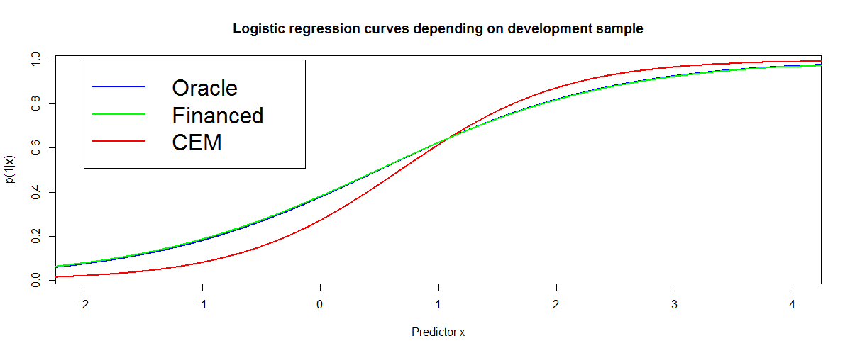
The cem algorithm is known for “sharpening” the decision boundary: predicted probabilities are closer to 0 and 1 than their true values as can be seen from simulated data from a MAR mechanism on Figure [2]. The scorecard \(\hat{\boldsymbol{\theta}}_{\text{f}}\) on financed clients (in green) is asymptotically consistent as was emphasized in Section 1.3.2 while the reclassified scorecard (in red) is biased even asymptotically.
Strategy 4: augmentation
Definition
Augmentation can be found in [36]. It is also documented as a “Re-Weighting method” in [46], [43] and [47]. This technique is directly influenced by the Importance Sampling [5] literature because intuitively, as for all selection mechanism such as survey respondents, observations should be weighted according to their probability of being in the sample w.r.t. the whole population, i.e. by \(p(z | \boldsymbol{x},y)\). By assuming implicitly a MAR missingness mechanism, as emphasized in Section 1.2.4, we get \(p(z | \boldsymbol{x}, y) = p(z | \boldsymbol{x})\).
For Credit Scoring practitioner, the estimate of interest is the mle of \(\ell(\boldsymbol{\theta};\mathcal{T} \cup \boldsymbol{\mathbf{y}}_{\text{nf}})\), which cannot be computed since we don’t know \(\boldsymbol{\mathbf{y}}_{\text{nf}}\). However we can derive the likelihood from the \(\text{KL}\) divergence by focusing on \(\mathbb{E}_{\boldsymbol{x},y} [\ln[p_{\boldsymbol{\theta}}(y|\boldsymbol{x})]]\). By noticing that \(p(\boldsymbol{x}) = \dfrac{p(\boldsymbol{x} | \text{f})}{p(\text{f} | \boldsymbol{x})} p(\text{f})\) and by assuming a MAR missingness mechanism, we get:
$$\mathbb{E}_{\boldsymbol{x},y} [\ln[p_{\boldsymbol{\theta}}(y|\boldsymbol{x})]] = p(\text{f}) \sum_{y=0}^1 \int_{\mathcal{X}} \dfrac{\ln p_{\boldsymbol{\theta}}(y | \boldsymbol{x})}{p(\text{f} | \boldsymbol{x})} p(y | \boldsymbol{x}) p(\boldsymbol{x} | \text{f}) d\boldsymbol{x} \approx_{n \to \infty} \dfrac{p(\text{f})}{n} \sum_{i \in \text{F}} \dfrac{1}{p(\text{f} | \boldsymbol{x}_i)} \ln p_{\boldsymbol{\theta}}(y_i | \boldsymbol{x}_i).$$
Consequently, had we access to \(p(\text{f} | \boldsymbol{x})\), the parameter maximizing the above mentioned likelihood would asymptotically be equal to the one on the through-the-door population, had we access to \(\boldsymbol{\mathbf{y}}_\text{nf}\). However, \(p(\text{f} | \boldsymbol{x})\) must be estimated by the practitioner’s method of choice, which will come with its bias and variance.
This method proposes to bin observations in \(\mathcal{T}\) in, say, 10 equal-length intervals of the score given by \(p_{\hat{\boldsymbol{\theta}}_\text{f}}(1 | \boldsymbol{x})\) and estimate \(p(z | \boldsymbol{x})\) as the proportion of financed clients in each of these bins. The inverse of this estimate is then used to weight financed clients in \(\mathcal{T}_{\text{f}}\) and retrain the model.
Missing data reformulation
The method aims at correcting for the selection procedure yielding the training data \(\mathcal{T}_{\text{f}}\) in the MAR case. As was argued in Section 1.3.2, if the model is well-specified, such a procedure is superfluous as the estimated parameter \(\hat{\boldsymbol{\theta}}_{\text{f}}\) is consistent. In the misspecified case however, it is theoretically justified as will be developed in the next paragraph. However, it is unclear if this apparent benefit is not offset by the added estimation procedure (which comes with its bias / variance trade-off).
Estimate property
The Importance Sampling paradigm requires \(p(\text{f} | \boldsymbol{x}) > 0\) for all \(\boldsymbol{x}\) which is clearly not the case here: for example, jobless people are never financed.
Strategy 5: twins
Definition
This reject inference method is documented internally at CACF; it consists in combining two scorecards: one predicting \(y\) learnt on financed clients (denoted by \(\hat{\boldsymbol{\theta}}_{\text{f}}\) as previously), the other predicting \(z\) learnt on all applicants, before learning the final scorecard using the predictions made by both scorecards on financed clients.
Missing data reformulation
The method aims at re-injecting information about the financing mechanism in the MAR missingness mechanism by estimating \(\hat{\boldsymbol{\phi}}\) as a logistic regression on all applicants, calculating scores \((1,\boldsymbol{x})' \hat{\boldsymbol{\theta}}_\text{f}\) and \((1,\boldsymbol{x})' \hat{\boldsymbol{\phi}}\) and use these as two continuous features in a third logistic regression predicting again the repayment feature \(y\).
Estimate property
It can be easily shown that this method is similar to the scorecard learnt on the financed clients.
Strategy 6: parcelling
Definition
The parcelling method can be found in . This method aims to correct the log-likelihood estimation in the MNAR case by making further assumptions on \(p(y | \boldsymbol{x}, z)\). It is a little deviation from the fuzzy augmentation method in a MNAR setting: we start with \(\hat{\boldsymbol{\theta}}^{(0)} = \hat{\boldsymbol{\theta}}_\text{f}\) and the practitioner arbitrarily decides to discretize the subsequent range of scores \((p_{\hat{\boldsymbol{\theta}}^{(0)} }(y_i | \boldsymbol{x}_i))_1^{n+n'}\) into, say, K scorebands B1, …, BK and “prudence factors” ϵ = (ϵ1, …, ϵK) generally such that 1 < ϵ1 < … < ϵK (non-financed low refunding probability clients are considered way riskier, all other things equal, than their financed counterparts). The method is thereafter strictly equivalent to fuzzy reclassification: a new logistic regression parameter is deduced from maximizing the expected complete log-likelihood as follows:
$$\hat{\boldsymbol{\theta}}^{(1)} = \arg\max_{\boldsymbol{\theta}} \mathbb{E}_{\boldsymbol{\mathbf{y}}_{\text{nf}}} [\ell_c(\boldsymbol{\theta};\mathcal{T}_{\text{c}}) | \mathcal{T},\hat{\boldsymbol{\theta}}^{(0)}, \boldsymbol{\epsilon}] = \ell(\boldsymbol{\theta};\mathcal{T}_{\text{f}}) + \sum_{i' = n + 1}^{n+n'} \epsilon_i p_{\hat{\boldsymbol{\theta}}^{(0)}}(y_i | \boldsymbol{x}_i) \ln p_{\boldsymbol{\theta}}(y_i | \boldsymbol{x}_i),$$
where \(\epsilon_i = \sum_{k=1}^K \epsilon_k \unicode{x1D7D9}(p_{\hat{\boldsymbol{\theta}}^{(0)}}(y_i | \boldsymbol{x}_i) \in B_k)\) is simply the prudence factor of each individual, depending on their scoreband, decided by the practitioner.
Missing data reformulation
By considering not-financed clients as riskier than financed clients with the same level of score, i.e. \(p(y | \boldsymbol{x}, \text{nf}) > p(y | \boldsymbol{x}, \text{f})\), it is implicitly assumed that manual operators (see Figure [1]) have access to additional information, say \(\tilde{\boldsymbol{x}}\) such as supporting documents, that influence the outcome \(y\) even when \(\boldsymbol{x}\) is accounted for. In this setting, rejected and accepted clients with the same score differ only by \(\tilde{\boldsymbol{x}}\), to which we do not have access and is accounted for “quantitatively” in a user-defined prudence factor ϵ stating that rejected clients would have been riskier than accepted ones.
Estimate property
The prudence factor encompasses the practitioner’s belief about the effectiveness of the operators’ rejections. It cannot be estimated from the data nor tested and is consequently a matter of unverifiable expert knowledge.
Numerical experiments
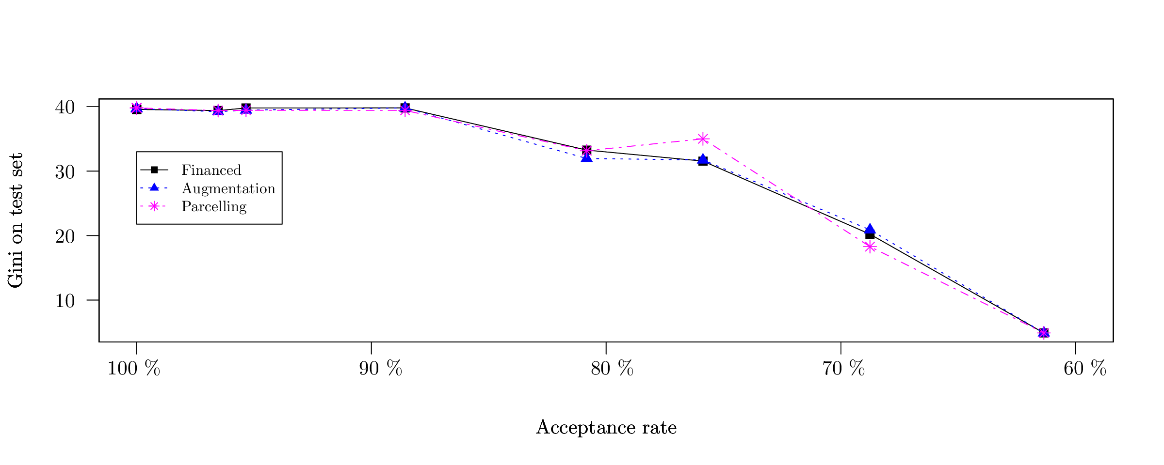
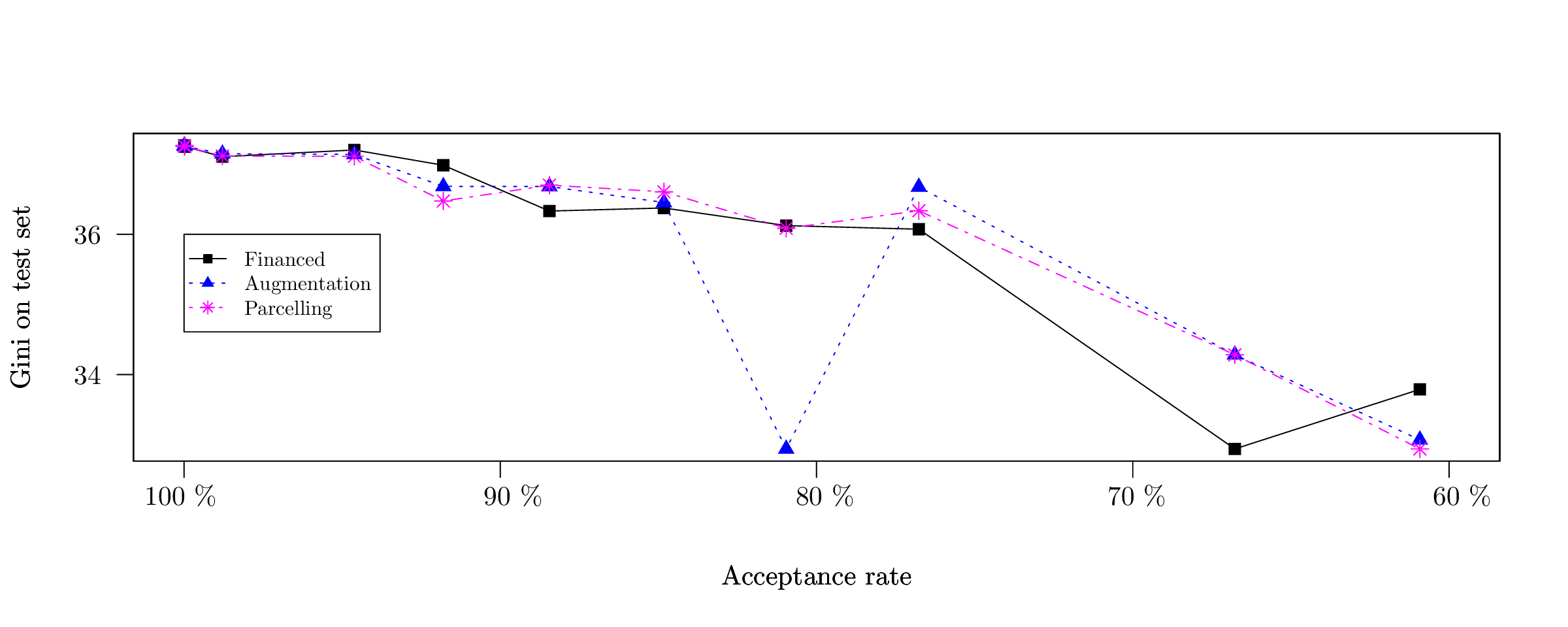
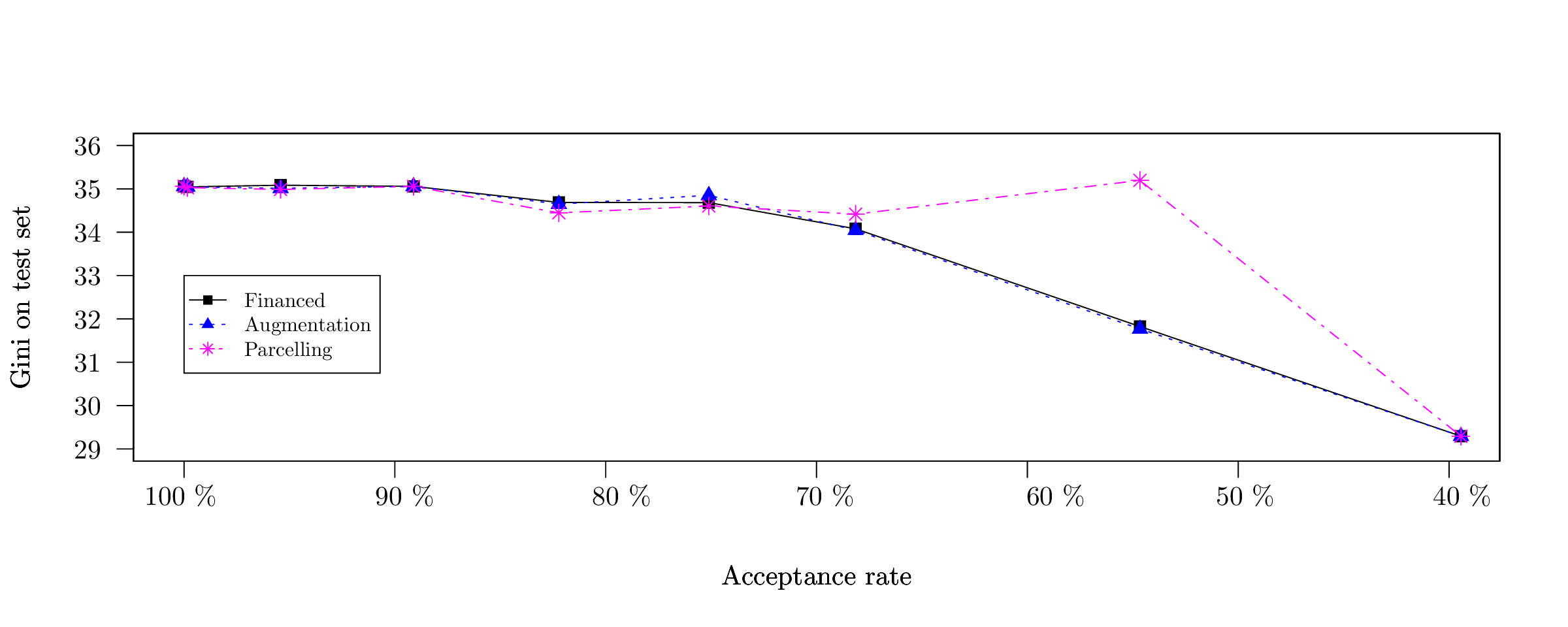
Here we focus on reject inference methods based on logistic regression applied to various CACF datasets: Electronics loans, Sports goods and Standard loans. They contain n = 180, 000, n = 35, 000 and n = 28, 000 respectively and d = 5, d = 8 and d = 6 categorical features with 3 to 10 levels per feature. The Electronics dataset consists in one year of financed clients through a partner of CACF that mainly sells electronics goods. The Sports dataset consists in one year of financed clients through a partner of CACF that sells all kinds of sports goods. The Standard consists in one year of financed clients stemming directly from sofinco.fr. The acceptance / rejection mechanism \(p_{\boldsymbol{\phi}}(z | \boldsymbol{x})\) is the existing scorecard and we simulate rejected applicants by progressively increasing the cut (the preceding threshold ϵ) of the existing scorecard.
The results in terms of Gini index are reported in Figure [3], [4] and [5] respectively. All methods perform relatively similarly and suffer from a big performance drop once the acceptance rate is below 50 % (at which point there are very few “bad borrower” events - y = 0). If we were to report 95 % confidence intervals around the Gini indices, we would get insignificant predictive performances, which confirms our theoretical findings.
Discussion: choosing the right model
Sticking with the financed clients model
Constructing scorecards by using a logistic regression on financed clients is a trade-off: on the one hand, it is implicitly assumed that it is well-specified, and that the missingness mechanism governing the observation of \(y\) is MAR. In other words, we suppose \(p(y | \boldsymbol{x}) = p_{\boldsymbol{\theta}^\star}(y | \boldsymbol{x}, \text{f})\). On the other hand, these assumptions, which seem strong at first hand, cannot really be relaxed: first, the use of logistic regression is a requirement from the financial institution. Second, the comparison of models cannot be performed using standard techniques since \(\boldsymbol{\mathbf{y}}_{\text{nf}}\) is missing (section 1.2.5). Third, strategies 4 and 6 that tackle the misspecified model and MNAR settings respectively require additional estimation procedures that, supplemental to their estimation bias and variance, take time from the practitioner’s perspective and are rather subjective (see sections 1.3.5 and 1.3.7), which is not ideal in the banking industry since there are auditing processes and model validation teams that might question these practices.
MCAR through a Control Group
Another simple solution often stated in the literature would be to keep a small portion of the population where applicants are not filtered: everyone gets accepted. This so-called Control Group would constitute the learning and test sets for all scorecard developments.
Although theoretically perfect, this solution faces a major drawback: it is costly, as many more loans will default. To construct the scorecard, a lot of data is required, so the minimum size of the Control Group is equivalent to a much bigger loss than the amount a bank would accept to lose to get a few more Gini points.
Keep several models in production: "champion challengers"
Several scorecards could also be developed, e.g. one using each reject inference technique. Each application is randomly scored by one of these scorecards. As time goes by, we would be able to put more weight on the most performing scorecard(s) and progressively less on the least performing one(s): this is the field of Reinforcement Learning .
The major drawback of this method, although its cost is very limited unlike the Control Group, is that it is very time-consuming for the credit modeller who has to develop several scorecards, for the IT who has to put them all into production, for the auditing process and for the regulatory institutions.
For years, the necessity of reject inference at CACF and other institutions (as it seems from the large literature coverage this research area has had) has been a question of personal belief. Moreover, there even exists contradictory findings in this area.
By formalizing the reject inference problem in section 1.2, we were able to pinpoint in which cases the current scorecard construction methodology, using only financed clients’ data, could be unsatisfactory: under a MNAR missingness mechanism and / or a misspecified model. We also defined criteria to reinterpret existing reject inference methods and assess their performance in Section 1.2.5. We concluded that no current reject inference method could enhance the current scorecard construction methodology: only the augmentation method (strategy 4) and the parcelling method (strategy 6) had theoretical justifications but introduce other estimation procedures. Additionally, they cannot be compared through classical model selection tools (Section 1.2.5).
We confirmed numerically these findings in the Appendices: given a true model and the MAR assumption, no logistic regression-based reject inference method performed best than the current method. In the misspecified model case, the Augmentation method seemed promising but it introduces a model that also comes with its bias and variance resulting in very close performances compared with the current method. With real data provided by CACF, we showed that all methods gave very similar results: the “best” method (by the Gini index) was highly dependent on the data and/or the proportion of unlabelled observations. Last but not least, in practice such a benchmark would not be tractable as \(\boldsymbol{\mathbf{y}}_{\text{nf}}\) is missing. In light of those limitations, adding to the fact that implementing those methods is a non-negligible time-consuming task, we recommend credit modellers to work only with financed loans’ data unless there is significant information available on either rejected applicants (\(\boldsymbol{\mathbf{y}}_{\text{nf}}\) - credit bureau information for example, which does not apply to France) or on the acceptance mechanism \(\boldsymbol{\phi}\) in the MNAR setting. On a side note, it must be emphasized that this work only applies to logistic regression and can be extended to all “local” models per the terminology introduced in [5]. For “global” models, e.g. decision trees, it can be shown that they are biased even in the MAR and well-specified settings, thus requiring ad hoc reject inference techniques such as an adaptation of the augmentation method (strategy 4 - see [5]).
All reject inference methods are detailed here.
Références
| [1] | Bradley Efron. The efficiency of logistic regression compared to normal discriminant analysis. Journal of the American Statistical Association, 70(352):892-898, 1975. [ bib ] |
| [2] | Rémi Lebret, Serge Iovleff, Florent Langrognet, Christophe Biernacki, Gilles Celeux, and Gérard Govaert. Rmixmod: the r package of the model-based unsupervised, supervised and semi-supervised classification mixmod library. Journal of Statistical Software, 67(6):241-270, 2014. [ bib ] |
| [3] |
Richard S. Sutton and Andrew G. Barto.
Reinforcement Learning: An Introduction.
The MIT Press, second edition, 2018.
[ bib |
.html ]
Keywords: 2018 book reference reinforcement-learning |
| [4] | Gilles Celeux and Gérard Govaert. A classification em algorithm for clustering and two stochastic versions. Computational statistics & Data analysis, 14(3):315-332, 1992. [ bib ] |
| [5] | Bianca Zadrozny. Learning and evaluating classifiers under sample selection bias. In Proceedings of the twenty-first international conference on Machine learning, page 114. ACM, 2004. [ bib ] |
| [6] |
Halbert White.
Maximum likelihood estimation of misspecified models.
Econometrica, 50(1):1-25, 1982.
[ bib |
http ]
This paper examines the consequences and detection of model misspecification when using maximum likelihood techniques for estimation and inference. The quasi-maximum likelihood estimator (OMLE) converges to a well defined limit, and may or may not be consistent for particular parameters of interest. Standard tests (Wald, Lagrange Multiplier, or Likelihood Ratio) are invalid in the presence of misspecification, but more general statistics are given which allow inferences to be drawn robustly. The properties of the QMLE and the information matrix are exploited to yield several useful tests for model misspecification.
|
| [7] |
Vincent Vandewalle.
Estimation et sélection en classification
semi-supervisée.
Theses, Université des Sciences et Technologie de Lille - Lille
I, December 2009.
[ bib |
http |
.pdf ]
Keywords: mixture models ; maximum likelihood estimation ; missing data ; EM algorithm ; discriminant analysis ; semi-supervised classification ; parsimonious models ; model choice ; modèles de mélange ; estimation par maximum de vraisemblance ; données manquantes ; algorithme EM ; analyse discriminante ; classification semi-supervisée ; modèles parcimonieux ; choix de modèle |
| [8] | Olivier Chapelle, Bernhard Schlkopf, and Alexander Zien. Semi-Supervised Learning. The MIT Press, 1st edition, 2010. [ bib ] |
| [9] | Stef Van Buuren, Hendriek C Boshuizen, Dick L Knook, et al. Multiple imputation of missing blood pressure covariates in survival analysis. Statistics in medicine, 18(6):681-694, 1999. [ bib ] |
| [10] | Roderick JA Little. Selection and pattern-mixture models. Longitudinal data analysis, pages 409-431, 2008. [ bib ] |
| [11] | Donald B Rubin. Multiple imputation for nonresponse in surveys, volume 81. John Wiley & Sons, 2004. [ bib ] |
| [12] | Stéphane Tufféry. Data mining et statistique décisionnelle : l'intelligence des données. Editions Technip, 2010. [ bib ] |
| [13] | Shaun Seaman, John Galati, Dan Jackson, John Carlin, et al. What is meant by “missing at random”? Statistical Science, 28(2):257-268, 2013. [ bib ] |
| [14] | Arthur P Dempster, Nan M Laird, and Donald B Rubin. Maximum likelihood from incomplete data via the em algorithm. Journal of the royal statistical society. Series B (methodological), pages 1-38, 1977. [ bib ] |
| [15] | Roderick JA Little. A test of missing completely at random for multivariate data with missing values. Journal of the American Statistical Association, 83(404):1198-1202, 1988. [ bib ] |
| [16] | Bradley Efron. The efficiency of logistic regression compared to normal discriminant analysis. Journal of the American Statistical Association, 70(352):892-898, 1975. [ bib ] |
| [17] | Terence J O'neill. The general distribution of the error rate of a classification procedure with application to logistic regression discrimination. Journal of the American Statistical Association, 75(369):154-160, 1980. [ bib ] |
| [18] | Crédit Groupe. Scorecard development methodology guidelines. Crédit Agricole Internal Guidelines, 2015. [ bib ] |
| [19] | Ricco Rakotomalala. Pratique de la régression logistique. Régression Logistique Binaire et Polytomique, Université Lumière Lyon, 2, 2011. [ bib ] |
| [20] | Halbert White. Maximum likelihood estimation of misspecified models. Econometrica: Journal of the Econometric Society, pages 1-25, 1982. [ bib ] |
| [21] | Joseph L Schafer and John W Graham. Missing data: our view of the state of the art. Psychological methods, 7(2):147, 2002. [ bib ] |
| [22] | Christophe Biernacki. Pourquoi les modèles de mélange pour la classification. Revue de MODULAD, 40:1-22, 2009. [ bib ] |
| [23] | Roderick JA Little and Donald B Rubin. Statistical analysis with missing data. John Wiley & Sons, 2014. [ bib ] |
| [24] | Bart Baesens. Developing intelligent systems for credit scoring using machine learning techniques. 2003. [ bib ] |
| [25] | Oleg Mazonka. Easy as : The importance sampling method. 2016. [ bib ] |
| [26] | Rémi Lebret, Serge Iovleff, Florent Langrognet, Christophe Biernacki, Gilles Celeux, and Gérard Govaert. Rmixmod: the r package of the model-based unsupervised, supervised and semi-supervised classification mixmod library. Journal of Statistical Software, pages In-press, 2015. [ bib ] |
| [27] | J. Ross Quinlan. C4.5: programs for machine learning. 1993. [ bib ] |
| [28] | Tin Kam Ho. Random decision forests. 1995. [ bib ] |
| [29] | Kevin Gurney. An introduction to neural networks. 1997. [ bib ] |
| [30] | Corinna Cortes and Vladimir Vapnik. Support-vector networks. 1995. [ bib ] |
| [31] | Gilles Celeux. The sem algorithm: a probabilistic teacher algorithm derived from the em algorithm for the mixture problem. Computational statistics quarterly, 2:73-82, 1985. [ bib ] |
| [32] | Christophe Biernacki, Gilles Celeux, and Gérard Govaert. Choosing starting values for the em algorithm for getting the highest likelihood in multivariate gaussian mixture models. Computational Statistics & Data Analysis, 41(3):561-575, 2003. [ bib ] |
| [33] | Geoffrey McLachlan and David Peel. Finite mixture models. John Wiley & Sons, 2004. [ bib ] |
| [34] | Jonathan Crook and John Banasik. Does reject inference really improve the performance of application scoring models? Journal of Banking & Finance, 28(4):857-874, April 2004. [ bib | DOI | http ] |
| [35] | G. Gongyue and Thomas. Bound and Collapse Bayesian Reject Inference When Data are Missing not at Random. [ bib | http ] |
| [36] | Emmanuel Viennet, Françoise Fogelman Soulié, and Benoît Rognier. Evaluation de techniques de traitement des refusés pour l'octroi de crédit. arXiv preprint cs/0607048, 2006. [ bib | http ] |
| [37] | D. J. Hand, K. J. McConway, and E. Stanghellini. Graphical models of applicants for credit. IMA Journal of Management Mathematics, 8(2):143-155, 1997. [ bib | http ] |
| [38] | James J. Heckman. Sample Selection Bias as a Specification Error. Econometrica, 47(1):153, January 1979. [ bib | DOI | http ] |
| [39] | Nicholas M. Kiefer and C. Erik Larson. Specification and informational issues in credit scoring. Available at SSRN 956628, 2006. [ bib | http ] |
| [40] | J. Banasik and J. Crook. Credit scoring, augmentation and lean models. Journal of the Operational Research Society, 56(9):1072-1081, 2005. [ bib | http ] |
| [41] | David J. Fogarty. Multiple imputation as a missing data approach to reject inference on consumer credit scoring. Interstat, 2006. [ bib | http ] |
| [42] | J. C. M. van Ophem, L. B. Gerlagh, and W. J. H. Verkooijen. Reject Inference in Credit Scoring. 2008. [ bib | http ] |
| [43] | John Banasik and Jonathan Crook. Reject inference, augmentation, and sample selection. European Journal of Operational Research, 183(3):1582-1594, 2007. [ bib | http ] |
| [44] | A. Feelders. Credit scoring and reject inference with mixture models. International Journal of Intelligent Systems in Accounting, Finance & Management, 9(1):1-8, 2000. [ bib | http ] |
| [45] | Corinna Cortes, Mehryar Mohri, Michael Riley, and Afshin Rostamizadeh. Sample selection bias correction theory. In International Conference on Algorithmic Learning Theory, pages 38-53. Springer, 2008. [ bib | http ] |
| [46] | Asma Guizani, Besma Souissi, Salwa Ben Ammou, and Gilbert Saporta. Une comparaison de quatre techniques d'inférence des refusés dans le processus d'octroi de crédit. In 45 emes Journées de statistique, 2013. [ bib | .pdf ] |
| [47] | Ha Thu Nguyen. Reject inference in application scorecards: evidence from France. Technical report, University of Paris West-Nanterre la Défense, EconomiX, 2016. [ bib | .pdf ] |
| [48] | Geert Molenberghs, Caroline Beunckens, Cristina Sotto, and Michael G Kenward. Every missingness not at random model has a missingness at random counterpart with equal fit. Journal of the Royal Statistical Society: Series B (Statistical Methodology), 7(2):371-388, 2008. [ bib ] |