Reject Inference - Appendix
N.B.: ce post s’inspire librement de mon manuscrit de thèse.
Fuzzy augmentation
Fuzzy augmentation can be found in [1]; it is the following procedure:
Construct Scorecard “Known Good Bad” (KGB) \(\hat{\boldsymbol{\theta}}_\text{f}\) with financed clients’ data (Figure [1a]);
Calculate \(p_{\hat{\boldsymbol{\theta}}_{\text{f}}}(1|\boldsymbol{\mathbf{x}}_{\text{nf}})\) for rejects (Figure [1b]);
Infer rejected client i as good with weight \(p_{\hat{\boldsymbol{\theta}}_{\text{f}}}(1|\boldsymbol{\mathbf{x}}_{\text{nf}})\) and as bad with weight
\(1-p_{\hat{\boldsymbol{\theta}}_{\text{f}}}(1|\boldsymbol{\mathbf{x}}_{\text{nf}})\) (Figures [1b] and [1c]);
Calibrate a new scorecard with the “augmented” dataset (Figure [1d]).
[1a]
| \({\boldsymbol{\mathbf{y}}}_{\text{f}}\) | \({\boldsymbol{\mathbf{x}}}_{\text{f}}\) |
|---|---|
| 1 | 0.562 |
| 1 | 0.910 |
| 0 | 0.430 |
[1b]
| Weight | \(\hat{\boldsymbol{\mathbf{y}}}_{\text{nf}}\) | \({\boldsymbol{\mathbf{x}}}_{\text{nf}}\) |
|---|---|---|
| 0.68 | 1 | 0.347 |
| 0.10 | 1 | 0.140 |
| 0.35 | 1 | 0.295 |
[1c]
| Weight | \(\hat{\boldsymbol{\mathbf{y}}}_{\text{nf}}\) | \({\boldsymbol{\mathbf{x}}}_{\text{nf}}\) |
|---|---|---|
| 0.32 | 0 | 0.347 |
| 0.90 | 0 | 0.140 |
| 0.65 | 0 | 0.295 |
[1d]
| Weight | \({\boldsymbol{\mathbf{y}}}\) | \({\boldsymbol{\mathbf{x}}}\) |
|---|---|---|
| 1 | 0 | 0.562 |
| 1 | 1 | 0.910 |
| 1 | 0 | 0.430 |
| 0.68 | 1 | 0.347 |
| 0.10 | 1 | 0.140 |
| 0.35 | 1 | 0.295 |
| 0.32 | 0 | 0.347 |
| 0.90 | 0 | 0.140 |
| 0.65 | 0 | 0.295 |
Clearly:
$$\forall j = 1, \ldots, d, \: \frac{\partial \sum_{i=n+1}^{m+n} \sum_{y_i = 0}^{1} p_{\hat{\boldsymbol{\theta}}_\text{f}}(y_i| \boldsymbol{x}_i)\ln (p_{\boldsymbol{\theta}}(y_i| \boldsymbol{x}_i))}{\partial \theta_j} = 0 \Leftrightarrow \theta = \hat{\boldsymbol{\theta}}_{\text{f}},$$
such that:
$$\arg\!\max_{\boldsymbol{\theta} \in \Theta} \sum_{i=n+1}^{m+n} \sum_{y_i = 0}^{1} p_{\hat{\boldsymbol{\theta}}_{\text{f}}}(y_i| \boldsymbol{x}_i)\ln (p_{\boldsymbol{\theta}}(y_i| \boldsymbol{x}_i)) = \hat{\boldsymbol{\theta}}_{\text{f}},$$
and finally:
$$\arg\!\max_{\boldsymbol{\theta} \in \Theta} \ell(\boldsymbol{\theta};\mathcal{T}_{c}) = \arg\!\max_{\boldsymbol{\theta} \in \Theta} \ell(\boldsymbol{\theta};\mathcal{T}_{\text{f}}) = \hat{\boldsymbol{\theta}}_{\text{f}}.$$
To conclude, this method will not change the estimated parameters of any discriminant model, asymptotically and with a finite set of observations, regardless of any assumption on the missingness mechanism or the true model hypothesis. In other words, Fuzzy Augmentation has no effect on the \(\text{KL}\) divergence, making this method useless because it is no different than the financed clients model.
Reclassification
Reclassification can be found in [2], also sometimes referred to as extrapolation as in [3]; it is the following procedure:
Construct Scorecard “Known Good Bad” (KGB) \(\hat{\boldsymbol{\theta}}_{\text{f}}\) with financed clients’ data (Figure [2a]);
Calculate \(p_{\hat{\boldsymbol{\theta}}_{\text{f}}}(1|\boldsymbol{x})\) for rejects;
Infer default status of rejected client i if \(p_{\hat{\boldsymbol{\theta}}_{\text{f}}}(1|\boldsymbol{x}) > \text{threshold}\); typically threshold = 0.5 (Figure [2b]);
Calibrate a new scorecard with the “augmented” dataset (Figure [2c]).
[2a]
| \({\boldsymbol{\mathbf{y}}}_{\text{f}}\) | \({\boldsymbol{\mathbf{x}}}_{\text{f}}\) |
|---|---|
| 1 | 0.562 |
| 1 | 0.910 |
| 0 | 0.430 |
[2b]
| \(p_{\hat{\boldsymbol{\theta}}_{\text{f}}}(1|\boldsymbol{\mathbf{x}})\) | \(\hat{\boldsymbol{\mathbf{y}}}_{\text{nf}}\) | \({\boldsymbol{\mathbf{x}}}_{\text{nf}}\) |
|---|---|---|
| 0.68 | 1 | 0.347 |
| 0.10 | 0 | 0.140 |
| 0.35 | 0 | 0.295 |
[2c]
| \({\boldsymbol{\mathbf{y}}}\) | \({\boldsymbol{\mathbf{x}}}\) |
|---|---|
| 0 | 0.562 |
| 1 | 0.910 |
| 0 | 0.430 |
| 1 | 0.347 |
| 0 | 0.140 |
| 0 | 0.295 |
Augmentation
Augmentation can be found in [2]. It is also documented as a “Re-Weighting method” in [4], [3] and [1].
Construct Scorecard “Accept Reject” (ACRJ) \(\hat{\boldsymbol{\phi}}\) with financed clients’ data on target variable Z (Figure [3a]);
Create K score bands B1, …, BK according to \(p_{\hat{\boldsymbol{\phi}}}(z | \boldsymbol{x})\);
Compute in each score band \(\hat{p}(\text{f}|p_{\hat{\boldsymbol{\phi}}}(z | \boldsymbol{x}) \in B_k) = \dfrac{|B_k|}{|\text{F}|}\) (Figure [3b]);
Construct a new scorecard on target variable Good/Bad with financed clients’ data re-weighted (Figure [3c]).
[3a]
| \({\boldsymbol{\mathbf{y}}}\) | z | Score-band |
|---|---|---|
| 1 | 1 | |
| 1 | 1 | |
| 0 | 1 | |
| NA | 1 | |
| NA | 1 | |
| NA | 1 | |
| ... | ... | ... |
[3b]
| Score-band | Weight | |
|---|---|---|
| 1 | 2 | |
| ... | ... | |
| K | 1.1 |
[3c]
| Weight | Score-band | \({\boldsymbol{\mathbf{y}}}\) | \({\boldsymbol{\mathbf{x}}}\) |
|---|---|---|---|
| 2 | 1 | 1 | 0.123 |
| 2 | 1 | 0 | 0.432 |
| 2 | 1 | 1 | 0.562 |
| ... | ... | ... | ... |
| 1.1 | K | 0 | 0.962 |
| 1.1 | K | 0 | 0.812 |
Twins
The twins method is an internal method at cacf documented in [5] (confidential) where Figure [4] is given; it consists in the following procedure:
Develop KGB (“Known Good/Bad”) scorecard \(\hat{\boldsymbol{\theta}}_\text{f}\) on financed clients’ data predicting \(\boldsymbol{\mathbf{y}}_\text{f}\) given \(\boldsymbol{\mathbf{x}}_\text{f}\) (Figure [5a]);
Develop ACRJ (Accept/Reject) scorecard \(\hat{\boldsymbol{\phi}}\) on all applicants predicting z given \(\boldsymbol{\mathbf{x}}\); this gives us \(\hat{\boldsymbol{\phi}}\) (Figure [5b]);
Develop a scorecard on financed clients’ data predicting \(\boldsymbol{\mathbf{y}}_\text{f}\) based solely on \((1,\boldsymbol{\mathbf{x}}_\text{f})' \hat{\boldsymbol{\theta}}_\text{f}\) and \((1,\boldsymbol{\mathbf{x}}_\text{f})' \hat{\boldsymbol{\phi}}\); this gives us \(\hat{\boldsymbol{\theta}}^{\text{twins}}\) (Figure [5c]);
Calculate \(p_{\hat{\boldsymbol{\theta}}^{\text{twins}}}(1 | \boldsymbol{x})\) on rejected applicants and reintegrate them twice in the training dataset like we did with fuzzy augmentation in Section 1.1 (Figure [5d]);
Develop a new scorecard on all applicants’ data.
[5a]
| \({\boldsymbol{\mathbf{y}}}\) | \({\boldsymbol{\mathbf{x}}}\) | |
|---|---|---|
| 1 | 0.562 | |
| 1 | 0.910 | |
| 0 | 0.430 | |
| NA | 0.361 | |
| NA | 0.402 | |
| NA | 0.294 |
[5b]
| z | \({\boldsymbol{\mathbf{x}}}\) | |
|---|---|---|
| 0.562 | ||
| 0.910 | ||
| 0.430 | ||
| 0.361 | ||
| 0.402 | ||
| 0.294 |
[5c]
| \({\boldsymbol{\mathbf{y}}}\) | \((1,\boldsymbol{\mathbf{x}}_\text{f})' \hat{\boldsymbol{\theta}}_\text{f}\) | \((1,\boldsymbol{\mathbf{x}}_\text{f})' \hat{\boldsymbol{\phi}}\) |
|---|---|---|
| 1 | 1.3 | 2.5 |
| 1 | 3.1 | 4.5 |
| 0 | -0.3 | 0.4 |
| NA | -1.2 | -0.5 |
| NA | -0.4 | 0.3 |
| NA | -2.0 | -2.5 |
[5d]
| Weight | \(\hat{\boldsymbol{\mathbf{y}}}_{\text{nf}}\) | \({\boldsymbol{\mathbf{x}}}_{\text{nf}}\) |
|---|---|---|
| 1 | 1 | 0.562 |
| 1 | 1 | 0.910 |
| 1 | 0 | 0.430 |
| 0.64 | 0 | 0.361 |
| 0.73 | 0 | 0.402 |
| 0.44 | 0 | 0.294 |
| 0.36 | 1 | 0.361 |
| 0.27 | 1 | 0.402 |
| 0.37 | 1 | 0.294 |
Following notations introduced in Chapter [chap2], we have:
$$\ell(\boldsymbol{\theta};(\boldsymbol{1},\boldsymbol{\mathbf{x}}_{\text{f}})' \hat{\boldsymbol{\phi}}, (\boldsymbol{1},\boldsymbol{\mathbf{x}}_{\text{f}})' \hat{\boldsymbol{\theta}}_\text{f}, \boldsymbol{\mathbf{y}}_{\text{f}}) = \sum_{i=1}^{n} \ln(p_{\boldsymbol{\theta}}(y_i | (1, \boldsymbol{x}_i)' \hat{\boldsymbol{\theta}}_{\text{f}}, (1, \boldsymbol{x}_i)' \hat{\boldsymbol{\phi}})).$$
We can rewrite \(\ell(\boldsymbol{\theta};(\boldsymbol{1},\boldsymbol{\mathbf{x}}_{\text{f}})' \hat{\boldsymbol{\phi}}, (\boldsymbol{1},\boldsymbol{\mathbf{x}}_{\text{f}})' \hat{\boldsymbol{\theta}}_\text{f}, \boldsymbol{\mathbf{y}}_{\text{f}})\) by remarking that the logit of \(p_{\boldsymbol{\theta}}(y_i | (1, \boldsymbol{x}_i)' \hat{\boldsymbol{\theta}}_{\text{f}}, (1, \boldsymbol{x}_i)' \hat{\boldsymbol{\phi}})\) is a linear combination of \(\boldsymbol{x}\). We know that \(\hat{\boldsymbol{\theta}}_{\text{f}} \in \arg\!\max_{\boldsymbol{\theta} \in \Theta} \ell(\boldsymbol{\theta};\boldsymbol{\mathbf{x}}_{\text{f}},\boldsymbol{\mathbf{y}}_{\text{f}})\) so that under the identifiability assumption, this method will give the same results as \(\hat{\boldsymbol{\theta}}^{\text{f}}\). In terms of \(\text{KL}\) divergence and as for Fuzzy Augmentation, this method is useless because it is no different than the financed clients model.
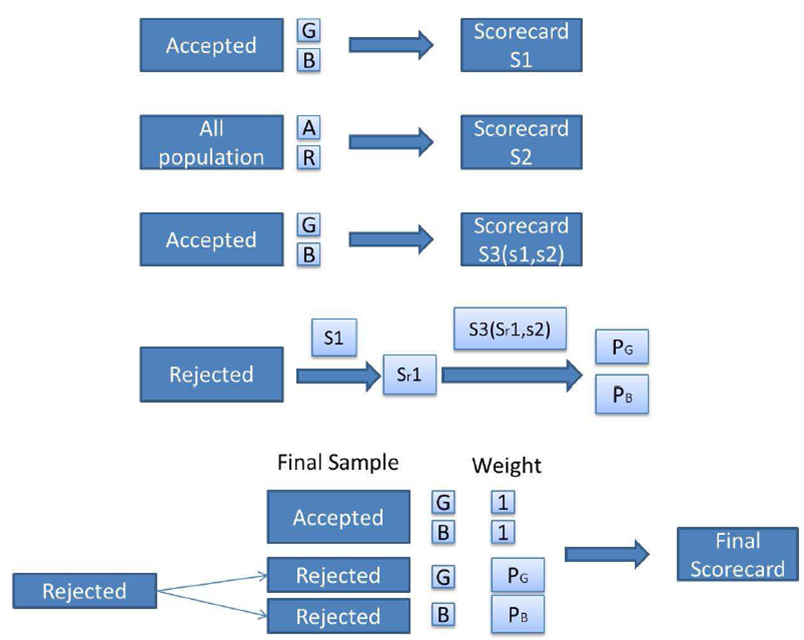
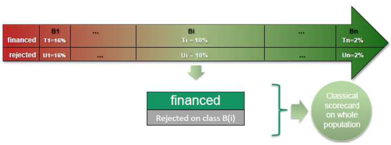
Parcelling
Parcelling is a process of reweighing according to the probability of default by score-band that is adjusted by the credit modeler. It has been documented in [4], [3] and [2], as well as in [5] where Figure [6] is given.
Construct Scorecard “Known Good Bad” (KGB) \(\hat{\boldsymbol{\theta}}_\text{f}\) with financed clients’ data (Figure [7a]);
Create K score bands B1, …, BK according to \(p_{\hat{\boldsymbol{\theta}}_\text{f}}(1 | \boldsymbol{x})\);
Compute the observed default rate for each band \(T(k) = \dfrac{|\text{Bad financed in } B_k|}{|B_k|}\), 1 ≤ k ≤ K;
Infer for each band the not financed default rate U(k) = ϵkT(k) where 1 < ϵ1 < … < ϵk < … < ϵK (Figure [7b]);
Reintegrate 2 times each rejected applicant from Bk with weight U(k) as bad and weight 1 − U(k) as good, like the Fuzzy Augmentation method in Section 1.1 (Figure [7c]);
Construct the final scorecard.
[7a]
| Weight | \({\boldsymbol{\mathbf{y}}}_{\text{f}}\) | \({\boldsymbol{\mathbf{x}}}_{\text{f}}\) |
|---|---|---|
| 1 | 1 | 0.562 |
| 1 | 1 | 0.910 |
| 1 | 0 | 0.430 |
[7b]
| Score-band | T | U |
|---|---|---|
| 1 | 0.5 | 0.8 |
| ... | ... | ... |
| K | 0.01 | 0.04 |
[7c]
| Weight | \({\boldsymbol{\mathbf{y}}}\) | \({\boldsymbol{\mathbf{x}}}\) |
|---|---|---|
| 1 | 0 | 0.562 |
| 1 | 1 | 0.910 |
| 1 | 0 | 0.430 |
| 1 | 1 | 0.347 |
| 1 | 0 | 0.140 |
| 1 | 0 | 0.295 |
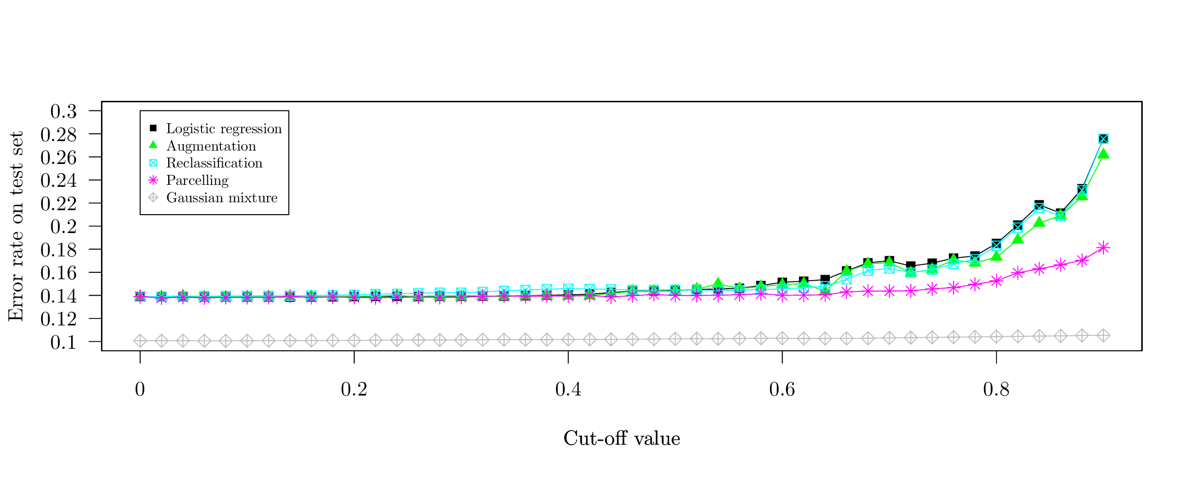
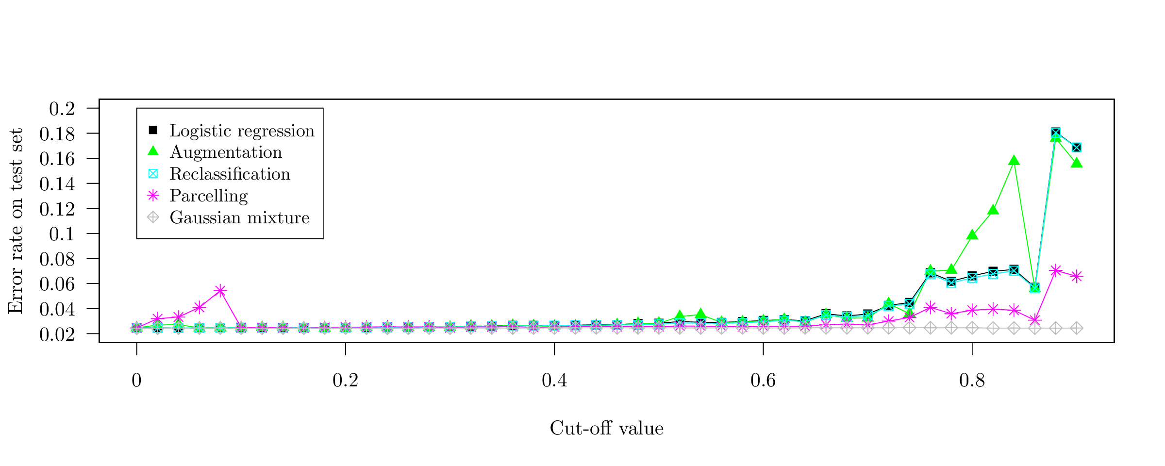
Simulation of reject inference methods applied to multivariate gaussian data
This early work aimed at comparing several reject inference methods in the well-specified model-case for 8 multivariate Gaussian features on Figure [fig:simu_4var] and 20 features on Figure [fig:simu_30var] in terms of error rate. The horizontal axis represents the cut-off value of a lr that simulates the acceptance / rejection mechanism \(p_{\boldsymbol{\phi}}(z | \boldsymbol{x})\), such that it roughly corresponds to the fraction of missing labels \(\boldsymbol{\mathbf{y}}_{\text{nf}}\). In this setting, the semi-supervised generative approach obviously yields better results since the data lies in its restricted hypothesis space and it is able to use the predictors with missing labels \(\boldsymbol{\mathbf{x}}_{\text{nf}}\). As explained thoroughly in Chapter [chap2], standard lr and Augmentation perform similarly (since they are both well-specified models and we are in a mar setting). Parcelling does not work well since it is designed for a mnar setting. In presence of well-separated data, Reclassification works well with 20 features since the true decision boundary is “sharp” (see the very small error rate) such that \(\arg\!\max_y \hat{p}(y | \boldsymbol{x}) \approx \max_y \hat{p}(y | \boldsymbol{x})\), which is less apparent with 8 features. In both cases, the mean of all features is 0 (resp. 1) if Y = 0 (resp. Y = 1) and the respective variance matrices are random positive definite matrices (see the Github repository of the manuscript at https://www.github.com/adimajo/manuscrit_these to reproduce them).
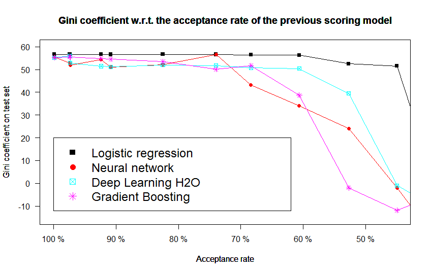
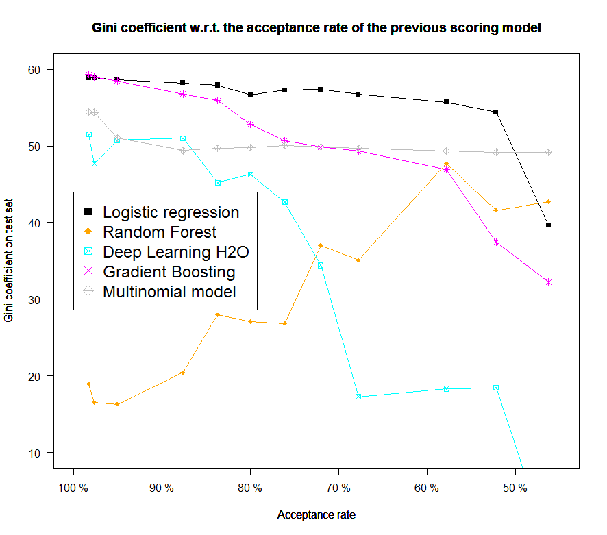
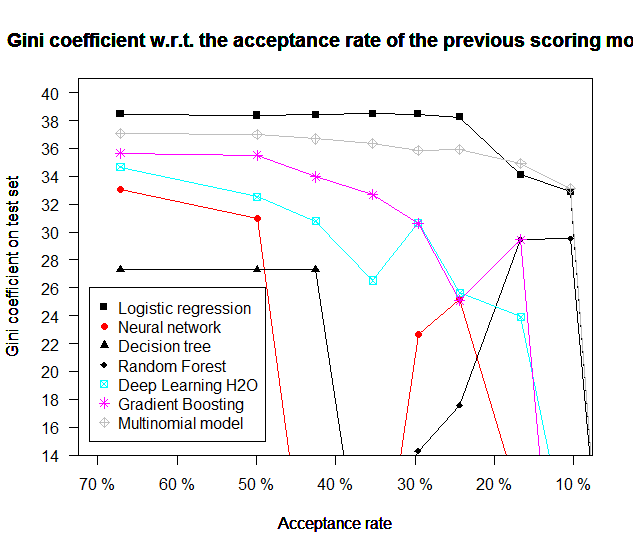
Performance of other predictive models w.r.t. the acceptance level
Also part of an earlier work, this section’s aim was to compare the performance of other “machine learning” models (although we purposely restricted our focus in Chapter [chap2] to the lr) to see if, when presented with the same data and in presence of a simulated acceptance / rejection mechanism as earlier showcased, it would not be of better interest to switch to a different model, although it was argued in Chapter [chap2] that these models would not perform good under a mar setting. The same datasets as in the previous section are used: the proposed models all perform poorer than lr but most importantly their performance drops significantly with the proportion of simulated accepted clients. Some studies of the reject inference problem have focused on these “machine learning” models.
[10]
[11]
[12]
Références
| [1] | Ha Thu Nguyen. Reject inference in application scorecards: evidence from France. Technical report, University of Paris West-Nanterre la Défense, EconomiX, 2016. [ bib | .pdf ] |
| [2] | Emmanuel Viennet, Françoise Fogelman Soulié, and Benoît Rognier. Evaluation de techniques de traitement des refusés pour l'octroi de crédit. arXiv preprint cs/0607048, 2006. [ bib | http ] |
| [3] | John Banasik and Jonathan Crook. Reject inference, augmentation, and sample selection. European Journal of Operational Research, 183(3):1582-1594, 2007. [ bib | http ] |
| [4] | Asma Guizani, Besma Souissi, Salwa Ben Ammou, and Gilbert Saporta. Une comparaison de quatre techniques d'inférence des refusés dans le processus d'octroi de crédit. In 45 emes Journées de statistique, 2013. [ bib | .pdf ] |
| [5] | Crédit Groupe. Scorecard development methodology guidelines. Crédit Agricole Internal Guidelines, 2015. [ bib ] |