Discretization and factor levels grouping in logistic regression
N.B.: ce post s’inspire librement de mon manuscrit de thèse.
To improve prediction accuracy and interpretability of logistic regression-based scorecards, a preprocessing step quantizing both continuous and categorical data is usually performed: continuous features are discretized by assigning factor levels to intervals and, if numerous, levels of categorical features are grouped. However, a better predictive accuracy can be reached by embedding this quantization estimation step directly into the predictive estimation step itself. By doing so, the predictive loss has to be optimized on a huge and intractable discontinuous quantization set. To overcome this difficulty, we introduced a specific two-step optimization strategy: first, the optimization problem is relaxed by approximating discontinuous quantization functions by smooth functions; second, the resulting relaxed optimization problem is solved either via a particular neural network and a stochastic gradient descent or an SEM algorithm. These strategies give then access to good candidates for the original optimization problem after a straightforward maximum a posteriori procedure to obtain cutpoints. The good performances of these approaches, which we call glmdisc-NN and glmdisc-SEM respectively, are illustrated on simulated and real data from the UCI library and CACF. The results show that practitioners finally have an automatic all-in-one tool that answers their recurring needs of quantization for predictive tasks.
Motivation
As stated in (1) and illustrated in this manuscript, in many application contexts (Credit Scoring, biostatistics, etc.), logistic regression is widely used for its simplicity, decent performance and interpretability in predicting a binary outcome given predictors of different types (categorical, continuous). However, to achieve higher interpretability, continuous predictors are sometimes discretized so as to produce a “scorecard”, i.e. a table assigning a grade to an applicant in Credit Scoring (or a patient in biostatistics, etc.) depending on its predictors being in a given interval, as exemplified in Table [1].
| Feature | Level | Points |
|---|---|---|
| Age | 18-25 | 10 |
| Age | 25-45 | 20 |
| Age | 45- + ∞ | 30 |
| Wages | − ∞-1000 | 15 |
| Wages | 1000-2000 | 25 |
| Wages | 2000- + ∞ | 35 |
| … | … | … |
Discretization is also an opportunity for reducing the (possibly large) modeling bias which can appear in logistic regression as a result of the linearity assumption on the continuous predictors in the model. Indeed, this restriction can be overcome by approximating the true predictive mapping with a step function where the tuning of the steps and their sizes allow more flexibility. However, the resulting increase of the number of parameters can lead to an increase in variance (overfitting) as shown in (2). Thus, a precise tuning of the discretization procedure is required. Likewise when dealing with categorical features which take numerous levels, their respective regression coefficients suffer from high variance. A straightforward solution formalized by (3) is to merge their factor levels which leads to less coefficients and therefore less variance. We showcase this phenomenon on simple simulated data in the next section. On Credit Scoring data, a typical example is the number of children (although not continuous strictly speaking). The log-odd ratio of clients’ creditworthiness w.r.t. their number of children is often visually “quadratic”, i.e. the risk is lower for clients having 1 to 3 children, a bit higher for 0 child, and then it grows steadily with the number of children above 4. This can be fitted with a parabola, see Figure [1]. As using a spline is not very interpretable, this is not done in practice. Without quantizing the number of children, a linear relationship is assumed as displayed on Figure [2]. When quantizing this feature, a piecewise constant relationship is assumed, see Figure [3]. In this example, it is visually unclear which is best, such that there is a need to formalize the problem.
Another potential motivation for quantization is optimal data compression: as will be shown rigorously in subsequent sections, quantization aims at “squeezing” as much predictive information in the original features about the class as possible. Taking an informatics point of view, quantization of a continuous feature is equivalent to discarding a float column (taking e.g. 32 bits per observation) by overwriting it with its quantized version (which would either be one column of unsigned 8 bits integers - “interval” encoding without order - or several 1 bit columns - one-hot / dummy encoding). The same thought process is applicable to quantizations of categorical features. In the end, the “raw” data can be compressed by a factor of 32/8 = 4 without losing its predictive power, which, in an era of Big Data, is useful both in terms of data storage and of computational power to process these data since by 2040, the energy needs for calculations will exceed the global energy production (see (4) p. 123).
From now on, the generic term quantization will stand for both discretization of continuous features and level grouping of categorical ones. Its aim is to improve the prediction accuracy. Such a quantization can be seen as a special case of representation learning , but suffers from a highly combinatorial optimization problem whatever the predictive criterion used to select the best quantization. The present work proposes a strategy to overcome these combinatorial issues by invoking a relaxed alternative of the initial quantization problem leading to a simpler estimation problem since it can be easily optimized by either a specific neural network or an SEM algorithm. These relaxed versions serve as a plausible quantization provider related to the initial criterion after a classical thresholding (maximum a posteriori) procedure.
The outline of this post is the following. After some introductory examples, we illustrate cases where quantization is either beneficial or detrimental depending on the data generating mechanism. In the subsequent section, we formalize both continuous and categorical quantization. Selecting the best quantization in a predictive setting is reformulated as a model selection problem on a huge discrete space which size is precisely derived. In Section 1.4, a particular neural network architecture is used to optimize a relaxed version of this criterion and propose good quantization candidates. In Section 1.5, an SEM procedure is proposed to solve the quantization problem. Section 1.6 is dedicated to numerical experiments on both simulated and real data from the field of Credit Scoring, high-lightening the good results offered by the use of the two new methods without any human intervention. A final section concludes the post by stating also new challenges.
![[fig:nbenf_spline] Risk of cacf clients w.r.t. their number of children and output of a spline regression.](figures/chapitre4/nbenf_spline.png)
![[fig:nbenf_cont] When the lr is used without quantization, it amounts to assuming the green linear relationship.](figures/chapitre4/nbenf_spline_cont.png)
![[fig:nbenf_disc] When the lr is used with quantization, e.g. more or less than 3 children, it amounts to assuming the risk is similar for all levels and equals the green steps.](figures/chapitre4/nbenf_spline_disc.png)
Illustration of the bias-variance quantization trade-off
The previous section motivated the use of quantization on a practical level. On a theoretical level, at least in terms of probability theory, quantization is equivalent to throwing away information: for continuous features, it is only known that they belong to a certain interval and for categorical features, their granularity among the original levels is lost.
However, two things must appear clearly: first, we are in a “statistical” setting, i.e. finite-dimensional setting, where variance of estimation can play a big role, which partly justifies the need to regroup categorical levels. Second, we are in a predictive setting, with an imposed classification model \(p_{\boldsymbol{\theta}}\). We focus on logistic regression, for which continuous features get a single coefficient: their relationship with the logit transform of the probability of an event (bad borrower) is assumed to be linear which can yield model bias. Thus, having several coefficients per feature, which can be achieved with a variety of techniques (e.g. splines), can yield a lower model bias (when the true model is not linear, which is generally the case for Credit Scoring data) at the cost of increased variance of estimation.
This phenomenon can be very simply captured by a small simulation: in the misspecified model setting, where the logit transform is assumed to stem from a sinusoidal transformation of \(x\) on [0; 1], it can clearly be seen from Figure [4a] that a standard linear logistic regression performs poorly. Discretizing the feature \(x\) results, using a very simple unsupervised heuristic named equal-length, in good results (i.e. visually mild bias / low variance) so long as the number of intervals, and subsequently of logistic regression coefficients, is low (see Figure [4b]). When the number of intervals gets large, the bias gets low (the sinus is well approximated by the little step functions), but the variance gets bigger (see Figure [4c]).
![[fig:sinus].](figures/chapitre4/fig_sinus.png)
As the number of intervals is directly linked to the number of coefficient, and to a notion of “complexity” of the resulting logistic regression model, the bias-variance trade-off plays a key role in choosing an appropriate step size, and, as will be seen in the next section which was not possible for the simple equal-length algorithm, appropriate step locations (hereafter called cutpoints). Again, this can be witnessed visually by looking at a model selection criterion, e.g. the BIC criterion, for different values of the number of intervals on Figure [5]. As expected, the continuous fit is poor, yielding a high BIC value. For a low number of bins, as described in the previous paragraph, the steps of are poor approximations of the true relationship between \(x\) and \(y\) resulting in a high BIC value. By discretizing in more intervals, the BIC value gets lower, and eventually starts to increase again when variance kicks in and overfitting occurs. As was visually concluded from the previous figure, somewhere around 10-15 intervals seem the most satisfactory since we clearly witness a low BIC value. Of course, as the model was misspecified, the flexibility brought by discretization was beneficial. The same phenomenon can be witnessed for categorical features on Figure [6] with real data from CACF. On Figure [6a], the logistic regression coefficients of the raw job types are displayed: none are significant and estimation variance is large. Grouping these levels results in narrower confidence intervals and significant logistic regression parameters as can be seen in Figure [6b]. We formalize these empirical findings in the next section.
![[fig:bic_sin].](figures/chapitre4/fig_bic_sin.png)
![[fig:csp].](figures/chapitre4/fig_csp.png)
Quantization as a combinatorial challenge
Quantization: definition
General principle
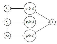
The quantization procedure consists in turning a d-dimensional raw vector of continuous and/or categorical features \(\boldsymbol{x} = (x_1, \ldots, x_d)\) into a d-dimensional categorical vector via a component-wise mapping \(\boldsymbol{q}=(\boldsymbol{q}_j)_1^d\):
$$\boldsymbol{q}(\boldsymbol{x})=(\boldsymbol{q}_1(x_1),\ldots,\boldsymbol{q}_d(x_d)).$$
Each of the univariate quantizations \(\boldsymbol{q}_j = (\boldsymbol{q}_{j,1}(x_j), \dots, \boldsymbol{q}_{j,m_j}(x_j)\) is a vector of \(m_j\) dummies:
$$\begin{align*}
& q_{j,h}(x_j) = 1 \text{ if } x_j \in C_{j,h}, 0 \text{ otherwise, } 1 \leq h \leq m_j, \\
& \boldsymbol{q}_j(\cdot) = e^h_{m_j} \end{align*}$$
where \(m_j\) is an integer, denoting the number of intervals / groups to which \(x_j\) is mapped and the sets Cj, h are defined with respect to each feature type as is described just below.
Raw continuous features
If \(x_j\) is a continuous component of \(\boldsymbol{x}\), quantization \(\boldsymbol{q}_j\) has to perform a discretization of \(x_j\) and the Cj, h’s, \(1 \leq h \leq m_j\), are contiguous intervals:
Cj, h = (cj, h − 1, cj, h],
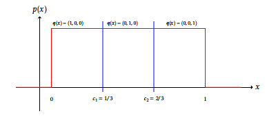
where \(c_{j,1},\ldots,c_{j,m_j-1}\) are increasing numbers called cutpoints, cj, 0 = − ∞, \(c_{j,m_j}=\infty\). For example, the quantization of the unit segment in thirds would be defined as \(m_j=3\), cj, 1 = 1/3, cj, 2 = 2/3 and subsequently \(\boldsymbol{q}_j(0.1) = (1,0,0)\). This is visually exemplified on Figure [7].
Raw categorical features
If \(x_j\) is a categorical component of \(\boldsymbol{x}\), quantization \(\boldsymbol{q}_j\) consists in grouping levels of \(x_j\) and the Cj, hs form a partition of the set \(\mathbb{N}_{o_j} = \{1, \dots, l_j\}\):
$$\begin{aligned}
%\bigsqcup_{h=1}^{m_j}C_{j,h}=\{1,\ldots,l_j\}.
\bigcup_{h=1}^{m_j}C_{j,h} & = \mathbb{N}_{o_j}, \\
\forall h, h', \: C_{j,h} \cap C_{j,h'} & = \varnothing .\end{aligned}$$
For example, the grouping of levels encoded as “1” and “2” would yield Cj, 1 = {1, 2} such that \(\boldsymbol{q}_j(1) = \boldsymbol{q}_j(2) = (1,0,\ldots,0)\). Note that it is assumed that there are no empty buckets, i.e. ∄j, h s.t. Cj, h = ⌀. This is visually exemplified on Figure [7].
![[fig:disc].](figures/chapitre4/fig_disc.png)
Cardinality of the quantization family
Notations for the quantization family
In both continuous and categorical cases, keep in mind that \(m_j\) is the dimension of \(\boldsymbol{q}_j\). For notational convenience, the (global) order of the quantization \(\boldsymbol{q}\) is set as
$$|\boldsymbol{q}|=\sum_{j=1}^d m_j.$$
The space where quantizations \(\boldsymbol{q}\) live (resp. \(\boldsymbol{q}_j\)) will be denoted by \(\boldsymbol{Q}_\boldsymbol{m}\) in the sequel (resp. \(\boldsymbol{Q}_j^{m_j}\)), when the number of levels \(\boldsymbol{m} = (m_j)_1^d\) is fixed. Since it is not known, the full model space is \(\boldsymbol{Q} = \cup_{m \in \mathbb{N}_\star^{d}} \boldsymbol{Q}_\boldsymbol{m}\) where \(\mathbb{N}_\star^{d} = (\mathbb{N} \setminus \{0\})^d\).
Equivalence of quantizations
Let \(\boldsymbol{q}^1\) and \(\boldsymbol{q}^2\) in \(\boldsymbol{Q}\) such that \(\boldsymbol{q}^1 \mathcal{R}_{\mathcal{T}_{\text{f}}} \boldsymbol{q}^2 \equiv \forall i,j \; \boldsymbol{q}^1_j(x_{i,j}) = \boldsymbol{q}^2_j(x_{i,j})\). See Figure [8] for an example.
![[fig:equiv].](figures/chapitre4/fig_equiv.png)
Lemma
Relation \(\mathcal{R}_{\mathcal{T}_{\text{f}}}\) defines an equivalence relation on \(\boldsymbol{Q}\).
Relation \(\mathcal{R}_{\mathcal{T}_{\text{f}}}\) is trivially reflexive and symmetric because of the reflexive and symmetric nature of the equality relation in \(\mathbb{R}\): \(\forall i,j \; \boldsymbol{q}^1_j(x_{i,j}) = \boldsymbol{q}^1_j(x_{i,j})\) and \(\forall i,j \; \boldsymbol{q}^1(x_{i,j}) = \boldsymbol{q}^2(x_{i,j})\). Similarly, let \(\boldsymbol{q}^3 \in \boldsymbol{Q}\) such that \(\boldsymbol{q}^1 \mathcal{R}_{\mathcal{T}_{\text{f}}} \boldsymbol{q}^3 \equiv \forall i,j \; \boldsymbol{q}^1_j(x_{i,j}) = \boldsymbol{q}^3_j(x_{i,j})\). Again, we immediately get \(\forall i,j \; \boldsymbol{q}^2_j(x_{i,j}) = \boldsymbol{q}^3_j(x_{i,j})\), i.e. \(\boldsymbol{q}^2 \mathcal{R}_{\mathcal{T}_{\text{f}}} \boldsymbol{q}^3\) which proves the transitivity of \(\mathcal{R}_{\mathcal{T}_{\text{f}}}\).
Cardinality of the quantization family in the continuous case
For a continuous feature xj, let \(\boldsymbol{q}_j \in \boldsymbol{Q}_j^{m_j}\) and cutpoints cj. Without any loss of generality, i.e. up to a relabelling on individuals i, it can be assumed that there are no empty intervals (all mj levels are observed) and consequently \(m_j+1\) observations \(x_{1,j},\dots,x_{m_j+1,j}\) s.t. \(x_{1,j} < c_{j,1} < x_{2,j} < \dots < c_{m_j-1,1} < x_{m_j+1,j}\). Indeed, if for example there exists \(k < m_j - 1\) s.t. \(c_{j,k} < \dots < c_{j,m_j-1}\) and max1 ≤ i ≤ nxi, j < cj, k, then discretization \(\boldsymbol{q}^{\text{bis}}_j \in \boldsymbol{Q}_{j,k}\) with k + 1 cutpoints ( − ∞, cj, 1, …, cj, k − 1, + ∞) is equivalent w.r.t. \(\mathcal{R}_{\mathcal{T}_n}\) to \(\boldsymbol{q}_j\): \(\forall i, \; \boldsymbol{q}_j(x_{i,j}) = \boldsymbol{q}^{\text{bis}}_j(x_{i,j})\). A similar proof can be conducted with cutpoints below the minimum of \(\boldsymbol{x}_j\) or with several cutpoints in-between consecutive values of the observations. Subsequently, there are \(\binom{n-1}{m_j-1}\) ways to construct cj, i.e. equivalence classes \([\boldsymbol{q}_j]\) for a fixed \(m_j \leq n\). The number of intervals \(m_j\) can range from 2 (binarization) to n (each xi, j is in its own interval, thus \(\boldsymbol{q}_j(x_{i,j}) \neq \boldsymbol{q}_j(x_{i',j})\) for i ≠ i′; ), so that the number of admissible discretizations of \(\boldsymbol{\mathbf{x}}_j\) is \(|\boldsymbol{Q}_j| = \sum_{i=2}^{n}\) \({n-1}\choose{i-1}\). Note that \(|\boldsymbol{Q}_j|\) depends on the number of observations n; we shall go back to this property in the following section.
Cardinality of the quantization family in the categorical case
For a continuous feature xj, let \(\boldsymbol{q}_j \in \boldsymbol{Q}_j\) with \(m_j\) groups. The number of re-arrangements of \(l_j\) labelled elements into \(m_j\) unlabelled groups is given by the Stirling number of the second kind \(S(l_j,m_j) = \frac{1}{m_j!} \sum_{i=0}^{m_j} (-1)^{m_j-i} {m_j \choose i} i^{l_j}\). As \(m_j\) is unknown, it must be searched over the range \(\{1,\dots,l_j\}\). Thus for categorical features, model space \(\boldsymbol{Q}_j\) is also discrete; subsequently, \(\boldsymbol{Q}\) is discrete.
Literature review
The current practice of quantization is prior to any predictive task, thus ignoring its consequences on the final predictive ability. It consists in optimizing a heuristic criterion, often totally unrelated (unsupervised methods) or at least explicitly (supervised methods) to prediction, and mostly univariate (each feature is quantized irrespective of other features’ values). The cardinality of the quantization space \(\boldsymbol{Q}\) was calculated explicitely w.r.t. d, \((m_j)_1^d\) and, for categorical features, \(l_j\): it is huge, so that a greedy approach is intractable and such heuristics are needed, as will be detailed in the next section.
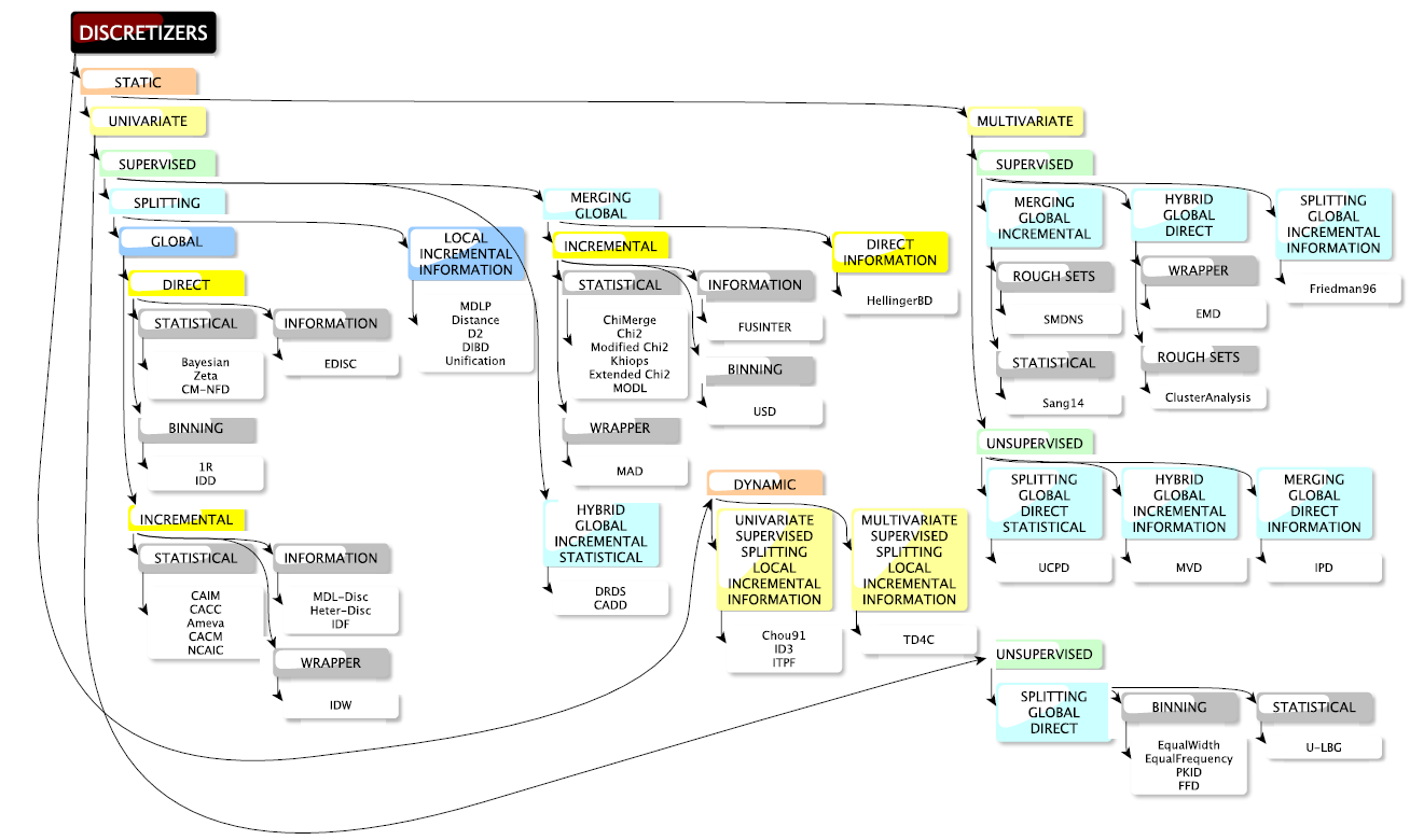
Many algorithms have thus been designed and a review of approximatively 200 discretization strategies, gathering both criteria and related algorithms, can be found in (5), preceded by other enlightening review articles such as (6), (7). They classify discretization methods by distinguishing, among other criteria and as said previously, unsupervised and supervised methods (y is used to discretize \(\boldsymbol{x}\)), for which model-specific (assumptions on \(p_{\boldsymbol{\theta}}\)) or model-free approaches are distinguished, univariate and multivariate methods (features \(\boldsymbol{x}_{-\{j\}} = (x_{1},\ldots,x_{j-1},x_{j+1},\ldots,x_{d})\) may influence the quantization scheme of \(x_j\)) and other criteria as can be seen from Figure [9] reproduced from (5) with permission.
For factor levels grouping, we found no such taxonomy, but some discretization methods, e.g. χ2 independence test-based methods can be naturally extended to this type of quantization, which is for example what the CHAID algorithm, proposed in (8) and applied to each categorical feature, relies on. A simple idea is also to use Group LASSO which attempts to shrink to zero all coefficients of a categorical feature to avoid situations where a few levels enter the model, which is arguably less interpretable. Another idea would be to use Fused LASSO , which seeks to shrink the pairwise absolute difference of selected coefficients, and apply it to all pairs of levels: the levels for which the difference would be shrunk to zero would be grouped. A combination of both approaches would allow both selection and grouping1.
For benchmarking purposes, and following results found in the taxonomy of (5), we used the MDLP (9) discretization method, which is a popular supervised univariate discretization method, and we implemented an extension of the discretization method ChiMerge (10) to categorical features, performing pairwise χ2 independence tests rather than only pairs of contiguous intervals, which we called ChiCollapse. Note that various refinements of ChiMerge have been proposed in the literature, Chi2 (11), ConMerge (12), ModifiedChi2 (13), and ExtendedChi2 (14), which seek to correct for multiple hypothesis testing (15) and automize the choice of the confidence parameter α in the χ2 tests, but adapting them to categorical features for benchmarking purposes would have been too time-consuming. A similar measure, called Zeta, has been proposed in place of χ2 in (16) and subsequent refinement (17): it is the classification error achievable by using only two contiguous intervals; if it is low, the two intervals are dissimilar w.r.t. the prediction task, if not, they can be merged.
Quantization embedded in a predictive process
In what follows, focus is given to logistic regression since it is a requirement from CACF but it is applicable to any other supervised classification model.
Logistic regression on quantized data
Quantization is a widespread preprocessing step to perform a learning task consisting in predicting, say, a binary variable \(y\in\{0,1\}\), from a quantized predictor \(\boldsymbol{q}(\boldsymbol{x})\), through, say, a parametric conditional distribution \(p_{\boldsymbol{\theta}}(y|\boldsymbol{q}(\boldsymbol{x}))\) like logistic regression; the whole process can be visually represented as a dependence structure among \(\boldsymbol{x}\), its quantization \(\boldsymbol{q}(\boldsymbol{x})\) and the target \(y\) on Figure [10]. Considering quantized data instead of raw data has a double benefit. First, the quantization order \(|\boldsymbol{q}|\) acts as a tuning parameter for controlling the model’s flexibility and thus the bias/variance trade-off of the estimate of the parameter \(\boldsymbol{\theta}\) (or of its predictive accuracy) for a given dataset. This claim becomes clearer with the example of logistic regression we focus on, as a still very popular model for many practitioners. On quantized data, logistic regression becomes:
$$\label{eq:reglogq}
\ln \left( \dfrac{p_{\boldsymbol{\theta}}(1|\boldsymbol{q}(\boldsymbol{x}))}{1 - p_{\boldsymbol{\theta}}(1|\boldsymbol{q}(\boldsymbol{x}))} \right) = \theta_0 + \sum_{j=1}^d \boldsymbol{q}_j(x_j)' \boldsymbol{\theta}_j,$$
where \(\boldsymbol{\theta} = (\theta_{0},(\boldsymbol{\theta}_j)_1^d) \in \mathbb{R}^{|\boldsymbol{q}|+1}\) and \(\boldsymbol{\theta}_j = (\theta_{j}^{1},\dots,\theta_{j}^{m_j})\) with \(\theta_{j}^{m_j} = 0\), j = 1…d, for identifiability reasons. Second, at the practitioner level, the previous tuning of \(|\boldsymbol{q}|\) through each feature’s quantization order \(m_j\), especially when it is quite low, allows an easier interpretation of the most important predictor values involved in the predictive process. Denoting the n-sample of financed clients by \((\boldsymbol{\mathbf{x}}_{\text{f}},\boldsymbol{\mathbf{y}}_{\text{f}})\), with \(\boldsymbol{\mathbf{x}}_{\text{f}}=(\boldsymbol{x}_1,\ldots,\boldsymbol{x}_n)\) and \(\boldsymbol{\mathbf{y}}_{\text{f}}=(y_1,\ldots,y_n)\), the log-likelihood
$$\label{eq:lq}
\ell_{\boldsymbol{q}}(\boldsymbol{\theta} ; \mathcal{T}_{\text{f}})=\sum_{i=1}^n \ln p_{\boldsymbol{\theta}}(y_i|\boldsymbol{q}(\boldsymbol{x}_i))$$
provides a maximum likelihood estimator \(\hat{\boldsymbol{\theta}}_{\boldsymbol{q}}\) of \(\boldsymbol{\theta}\) for a given quantization \(\boldsymbol{q}\). For the rest of the post, the approach is exemplified with logistic regression as \(p_{\boldsymbol{\theta}}\) but it can be applied to any other predictive model, as will be recalled in the concluding section.
Quantization as a model selection problem
As dicussed in the previous section, and emphasized in the literature review, quantization is often a preprocessing step; however, quantization can be embedded directly in the predictive model. Continuing our logistic example, a standard information criteria such as the BIC can be used to select the best quantization:
$$\label{eq:BICq}
\hat{\boldsymbol{q}}=\arg\!\min_{\boldsymbol{q} \in \boldsymbol{Q}} \text{BIC}(\hat{\boldsymbol{\theta}}_{\boldsymbol{q}})$$
where the “complexity” parameter depends on \({\boldsymbol{q}}\) and is traditionally the number of continuous parameters to be estimated in the \(\boldsymbol{\theta}\)-parameter space. The practitioner can swap this criterion with any other penalized criterion on training data such as AIC (18) or, as Credit Scoring people like, the Gini index on a test set. Note however that, regardless of the used criterion, an exhaustive search of \(\hat{\boldsymbol{q}}\in\boldsymbol{Q}\) is an intractable task due to its highly combinatorial nature as was explicitly formulated in the previous section. Anyway, the optimization of the above BIC criterion requires a new specific strategy that is described in the next section.
Remarks on model selection consistency
In high-dimensional spaces and among models with a wildly varying number of parameters, classical model selection tools like BIC can have disappointing asymptotic properties, as emphasized in (19), where a modified BIC criterion, taking into account the number of models per parameter size, is proposed. Moreover in essence, as is apparent from the \(\hat{\boldsymbol{\theta}}_{\boldsymbol{q}}\) symbol, and supplemental to the logistic regression coefficients per se, the inherent “parameters” Cj, h of \(\boldsymbol{q}\) shall be accounted for in the penalization term ν: they are estimated indirectly in all quantization methods, and in particular in the one we propose in the subsequent section.
In addition, the BIC criterion relies on the Laplace approximation which requires the likelihood to be twice differentiable in the parameters. However, as \(\boldsymbol{q}\) consists in a collection of step functions of parameters Cj, h, this is not the case. For continuous features, since it is nevertheless almost everywhere differentiable, for the properties of the BIC criterion to hold, it suffices that there exists a neighbourhood Vj, h around true parameters cj, h⋆ where there is no observation: \(\not\exists i, \: x_{i,j} \in V_{j,h}\). For categorical features, the Laplace approximation is no longer valid and there is no way, in general, to approximate the integral (i.e. the sum over the discrete parameter space) by “counting” the number of parameters as in the continuous case (20).
The proposed neural network based quantization
A relaxation of the optimization problem
In this section, we propose to relax the constraints on \(\boldsymbol{q}_j\) to simplify the search of \(\hat{\boldsymbol{q}}\). Indeed, the derivatives of \(\boldsymbol{q}_j\) are zero almost everywhere and consequently a gradient descent cannot be directly applied to find an optimal quantization.
Smooth approximation of the quantization mapping
A classical approach is to replace the binary functions qj, h by smooth parametric ones with a simplex condition, namely with \(\boldsymbol{\alpha}_j=(\boldsymbol{\alpha}_{j,1},\ldots, \boldsymbol{\alpha}_{j,m_j})\):
$$%\label{eq:qaj}
{\boldsymbol{q}_{\boldsymbol{\alpha}_j}(\cdot)=\left(q_{\boldsymbol{\alpha}_{j,h}}(\cdot)\right)_{h=1}^{m_j} \text{ with } \sum_{h=1}^{m_j}q_{\boldsymbol{\alpha}_{j,h}}(\cdot)=1 \text{ and } 0 \leq q_{\boldsymbol{\alpha}_{j,h}}(\cdot) \leq 1,}$$
where functions \(q_{\boldsymbol{\alpha}_{j,h}}(\cdot)\), properly defined hereafter for both continuous and categorical features, represent a fuzzy quantization in that, here, each level h is weighted by \(q_{\boldsymbol{\alpha}_{j,h}}(\cdot)\) instead of being selected once and for all. The resulting fuzzy quantization for all components depends on the global parameter \(\boldsymbol{\alpha} = (\boldsymbol{\alpha}_1, \ldots, \boldsymbol{\alpha}_d)\) and is denoted by \(\boldsymbol{q}_{\boldsymbol{\alpha}}(\cdot)=\left(\boldsymbol{q}_{\boldsymbol{\alpha}_j}(\cdot)\right)_{j=1}^d\).
For continuous features, we set for \(\boldsymbol{\alpha}_{j,h} = (\alpha^0_{j,h},\alpha^1_{j,h}) \in \mathbb{R}^2\)
$$\label{eq:softmax}
q_{\boldsymbol{\alpha}_{j,h}}(\cdot) = \frac{\exp(\alpha^0_{j,h} + \alpha^1_{j,h} \cdot)}{\sum_{g=1}^{m_j} \exp(\alpha^0_{j,g} + \alpha^1_{j,g} \cdot)}$$
where \(\boldsymbol{\alpha}_{j,m_j}\) is set to (0, 0) for identifiability reasons.
For categorical features, we set for \(\boldsymbol{\alpha}_{j,h}=\left(\alpha_{j,h}(1),\ldots, \alpha_{j,h}(l_j)\right) \in \mathbb{R}^{l_j}\)
$$q_{\boldsymbol{\alpha}_{j,h}}(\cdot) = \frac{\exp\left(\alpha_{j,h}(\cdot)\right)}{\sum_{g=1}^{m_j} \exp\left(\alpha_{j,g}(\cdot)\right)}$$
where \(l_j\) is the number of levels of the categorical feature \(x_j\).
Parameter estimation
With this new fuzzy quantization, the logistic regression for the predictive task is then expressed as
$$\label{eq:reglogqa}
\ln \left( \dfrac{p_{\boldsymbol{\theta}}(1|\boldsymbol{q}_{\boldsymbol{\alpha}} (\boldsymbol{x}))}{1 - p_{\boldsymbol{\theta}}(1|\boldsymbol{q}_{\boldsymbol{\alpha}} (\boldsymbol{x}))} \right) = \theta_0 + \sum_{j=1}^d { \boldsymbol{q}_{\boldsymbol{\alpha}_{j}}(x_j)' \boldsymbol{\theta}_j },$$
where \(\boldsymbol{q}\) has been replaced by \(\boldsymbol{q}_{\boldsymbol{\alpha}}\). Note that as \(\boldsymbol{q}_{\boldsymbol{\alpha}}\) is a sound approximation of \(\boldsymbol{q}\) (see above), this logistic regression in \(\boldsymbol{q}_{\boldsymbol{\alpha}}\) is consequently a good approximation of the logistic regression in \(\boldsymbol{q}\). The relevant log-likelihood is here
$$\label{eq:lqa}
\ell_{\boldsymbol{q}_{\boldsymbol{\alpha}}}(\boldsymbol{\theta} ; \mathcal{T}_{\text{f}})=\sum_{i=1}^n \ln p_{\boldsymbol{\theta}}(y_i|\boldsymbol{q}_{\boldsymbol{\alpha}}(\boldsymbol{x}_i))$$
and can be used as a tractable substitute for \(\ell_q\) to solve the original optimization problem, where now both \(\boldsymbol{\alpha}\) and \(\boldsymbol{\theta}\) have to be estimated, which is discussed in the next section.
Deducing quantizations from the relaxed problem
We wish to maximize the log-likelihood \(\ell_{\boldsymbol{q}_{\boldsymbol{\alpha}}}\) which would yield parameters \((\hat{\boldsymbol{\alpha}},\hat{\boldsymbol{\theta}})\); these are consistent if the model is well-specified (i.e. there is a “true” quantization under classical regularity conditions). Denoting by A the space of \(\boldsymbol{\alpha}\) and \(\boldsymbol{Q}_A\) the space of \(\boldsymbol{q}_{\boldsymbol{\alpha}}\), to “push” \(\boldsymbol{Q}_A\) further into \(\boldsymbol{Q}\), \(\hat{\boldsymbol{q}}\) is deduced from a maximum a posteriori procedure applied to \(\boldsymbol{q}_{\hat{\boldsymbol{\alpha}}}\):
$$\label{eq:ht}
\hat{q}_{j,h}(x_j) = 1 \equiv \hat{\boldsymbol{q}}_j(x_j) = e^h_{m_j} \text{ if } h = \arg\!\max_{1 \leq h' \leq m_j} q_{\hat{\boldsymbol{\alpha}}_{j,h'}}(x_j), 0 \text{ otherwise.}
%\nonumber$$
If there are several levels h that satisfy the above argmax, we simply take the level that corresponds to smaller values of \(x_j\) to be in accordance with the definition of Cj, h. This maximum a posteriori principle will be exemplified in Figure [11] on simulated data. These approximations are justified by the following arguments.
Rationale
From a deterministic point of view, we have \(\boldsymbol{Q} \subset \boldsymbol{Q}_A\): First, the maximum a posteriori step produces contiguous intervals (i.e. there exists Cj, h; 1 ≤ j ≤ d, \(1 \leq h \leq m_j\), s.t. \({\hat{\boldsymbol{q}}}\) can be written as a proper quantization (21). Second, in the continuous case, the higher αj, h1, the less smooth the transition from one quantization h to its “neighbor” h + 1, whereas \(\dfrac{\alpha_{j,h}^0}{\alpha_{j,h}^1}\) controls the point in \(\mathbb{R}\) where the transition occurs (22). Concerning the categorical case, the rationale is even simpler as \(q_{\lambda \boldsymbol{\alpha}_j}(x_j) \to e^h_{m_j} \text{ if } h = \arg\!\max_{h'} q_{\alpha_{j,h'}}(x_j)\) as λ → + ∞ (23).
From a statistical point of view, provided the model is well-specified, i.e.:
$$\label{eq:well_quant}
\exists \boldsymbol{q}^\star, \boldsymbol{\theta}^\star, \forall \boldsymbol{x},y, \; p(y | \boldsymbol{x}) = p_{\boldsymbol{\theta}^\star}(y | \boldsymbol{x});$$
and under standard regularity conditions and with a suitable estimation procedure (see later for the proposed estimation procedure), the maximum likelihood framework would ensure the consistency of \((\boldsymbol{q}_{\hat{\boldsymbol{\alpha}}}, \hat{\boldsymbol{\theta}})\) towards \((\boldsymbol{q}^\star,\boldsymbol{\theta}^\star)\) if \(\boldsymbol{\alpha}^\star\) s.t. \(\boldsymbol{q}_{\boldsymbol{\alpha}^\star} = \boldsymbol{q}\) was an interior point of the parameter space A. However, as emphasized in the previous paragraph, “\(\boldsymbol{\alpha}^\star = + \infty\)” such that the maximum likelihood parameter is on the edge of the parameter space which hinders asymptotic properties (e.g. normality) in some settings (24), but not “convergence” on which we focus here. We did not investigate this issue further since numerical experiments showed consistency: from an empirical point of view, we will see in Section 1.6 and in particular in Figure [11], that the smooth approximation \(\boldsymbol{q}_{\hat{\boldsymbol{\alpha}}}\) converges towards “hard” quantizations \(\boldsymbol{q}\).
However, and as is usual, the log-likelihood \(\ell_{\boldsymbol{q}_{\boldsymbol{\alpha}}}(\boldsymbol{\theta},(\boldsymbol{\mathbf{x}},\boldsymbol{\mathbf{y}}))\) cannot be directly maximized w.r.t. \((\boldsymbol{\alpha},\boldsymbol{\theta})\), so that we need an iterative procedure. To this end, the next section introduces a neural network of suitable architecture.
A neural network-based estimation strategy
Neural network architecture
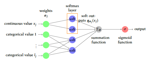
To estimate parameters \(\boldsymbol{\alpha}\) and \(\boldsymbol{\theta}\) in the relaxed logistic regression model, a particular neural network architecture can be used. We shall insist that this network is only a way to use common deep learning frameworks, namely Tensorflow (25) through the high-level API Keras (26) instead of building a gradient descent algorithm from scratch to optimize \(\ell_{\boldsymbol{q}_{\boldsymbol{\alpha}}}(\boldsymbol{\theta},(\boldsymbol{\mathbf{x}},\boldsymbol{\mathbf{y}}))\). The most obvious part is the output layer that must produce \(p_{\boldsymbol{\theta}}(1|\boldsymbol{q}_{\boldsymbol{\alpha}}(\boldsymbol{x}))\) which is equivalent to a densely connected layer with a sigmoid activation (the reciprocal function of logit).
For a continuous feature \(x_j\) of \(\boldsymbol{x}\), the combined use of \(m_j\) neurons including affine transformations and softmax activation obviously yields \(\boldsymbol{q}_{\boldsymbol{\alpha}_{j}}(x_j)\). Similarly, an input categorical feature \(x_j\) with \(l_j\) levels is equivalent to \(l_j\) binary input neurons (presence or absence of the factor level). These \(l_j\) neurons are densely connected to \(m_j\) neurons without any bias term and a softmax activation. The softmax outputs are next aggregated via the summation, say \(\Sigma_{\boldsymbol{\theta}}\) for short, and then the sigmoid function σ gives the final output. All in all, the proposed model is straightforward to optimize with a simple neural network, as shown in Figure [12].
Stochastic gradient descent as a quantization provider
By relying on stochastic gradient descent, the smoothed likelihood \(\ell_{\boldsymbol{q}_{\boldsymbol{\alpha}}}(\boldsymbol{\theta},(\boldsymbol{\mathbf{x}},\boldsymbol{\mathbf{y}}))\) can be maximized over \(\left(\boldsymbol{\alpha}, \boldsymbol{\theta} \right)\). Due to its convergence properties (27), the results should be close to the maximizers of the original likelihood \(\ell_{\boldsymbol{q}}\) if the model is well-specified, when there is a true underlying quantization. However, in the misspecified model case, there is no such guarantee. Therefore, to be more conservative, we evaluate at each training epoch (s) the quantization \(\hat{\boldsymbol{q}}^{(s)}\) resulting from the maximum a posteriori procedure, then classically estimate the logistic regression parameter via maximum likelihood:
$$\label{eq:lr_param_q}
\hat{\boldsymbol{\theta}}^{(s)} = \arg\!\max_{\boldsymbol{\theta}} \ell_{\hat{q}^{(s)}}(\boldsymbol{\theta}; \mathcal{T}_{\text{f}})$$
and the resulting \(\mbox{BIC}(\hat{\boldsymbol{\theta}}^{(s)})\). If S is a given maximum number of iterations of the stochastic gradient descent algorithm, the quantization retained at the end is then determined by the optimal epoch
$$\label{eq:opt_epoch}
s^\star=\arg\!\min_{s\in \{1,\ldots, S\}} \mbox{BIC}(\hat{\boldsymbol{\theta}}^{(s)}).$$
You can think of S as a computational budget: contrary to classical early stopping rules (e.g. based on validation loss) used in neural network fitting, this network only acts as a stochastic quantization provider which will naturally prevent overfitting. We reiterate that the BIC can be swapped for the user’s favourite model choice criterion.
Lots of optimization algorithms for neural networks have been proposed, which all come with their hyperparameters. As, in the general case, \(\ell_{\boldsymbol{q}_{\boldsymbol{\alpha}}}(\boldsymbol{\theta} ; (\boldsymbol{\mathbf{x}},\boldsymbol{\mathbf{y}}))\) is not guaranteed to be convex, there might be several local maxima, such that all these optimization methods might diverge, converge to a different maximum, or at least converge in very different numbers of epochs, as is examplified on this Github repo2. We chose the RMSProp method, which showed good results and is one of the standard methods.
Choosing an appropriate number of levels
Concerning now the number of intervals or factor levels \(\boldsymbol{m} = (m_j)_1^d\), they have also to be estimated since in practice they are unknown. Looping over all candidates m is intractable. But in practice, by relying on the maximum a posteriori procedure, a lot of unseen factor levels might be dropped. Indeed, for a given level h, all training observations \(x_{i,j}\) in \(\mathcal{T}_{\text{f}}\) and all other levels h′, if \(q_{\boldsymbol{\alpha}_{j,h}}(x_{i,j}) < q_{\boldsymbol{\alpha}_{j,h'}}(x_{i,j})\), then the level h “vanishes”.
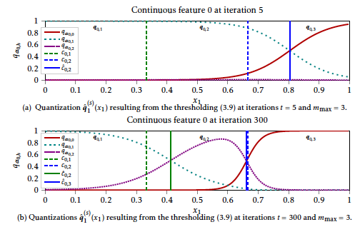
This phenomenon can be witnessed in Figure [11] (algorithm and experiments detailed later) where qα0, 2 is “flat” across the support of \(\boldsymbol{\mathbf{x}}_0\) and only two intervals are produced. In practice, we recommend to start with a user-chosen \(\boldsymbol{m}=\boldsymbol{m}_{\max}\) and we will see in the experiments of Section 1.6 that the proposed approach is able to explore small values of m and to select a value \(\hat{\boldsymbol{m}}\) drastically smaller than mmax. This phenomenon, which reduces the computational burden of the quantization task, is also illustrated in Section 1.6.
An alternative SEM approach
In what follows, the quantization \(\boldsymbol{q}(\boldsymbol{x})\) is seen as a latent (unobserved) feature denoted by \(\boldsymbol{\mathfrak{q}}\), which is still the vector of quantizations \((\boldsymbol{\mathfrak{q}}_1, \dots, \boldsymbol{\mathfrak{q}}_d)\) of features \((x_1, \dots, x_d)\). These component-wise quantizations are themselves binary-valued vectors \((\mathfrak{q}_{j,h})_1^{m_j}\) where 𝔮j, h ∈ {0, 1} and \(\sum_{h=1}^{m_j} \mathfrak{q}_{j,h} = 1\). We denote by \(\boldsymbol{\mathfrak{Q}}_{\boldsymbol{m}}\) the space of such latent features and the n-sample of latent quantizations corresponding to \(\boldsymbol{q}(\boldsymbol{\mathbf{x}}_\text{f})\) by \(\boldsymbol{\mathbf{q}}\), i.e. the matrix of all n quantizations.
In the following section, we translate earlier assumptions on the function \(\boldsymbol{q}(\cdot)\) in probabilistic terms for the latent featutre \(\boldsymbol{\mathfrak{q}}\). In the subsequent section, we make good use of these assumptions to provide a continuous relaxation of the quantization problem, as was empirically argumented in Section 1.4.1. The main reason to resort to this formulation as a latent feature problem will be made clear in Section 1.5.3, where we provide a stochastic estimation algorithm for the latent feature \(\boldsymbol{\mathfrak{q}}\).
Probabilistic assumptions regarding the quantization latent feature
Firstly, only the well-specified model case is considered. This hypothesis translates with this new latent feature as a probabilistic assumption:
$$\label{hyp:true}
\exists \boldsymbol{\theta}^\star, \boldsymbol{\mathfrak{q}}^\star \text{s.t.} Y \sim p_{\boldsymbol{\theta}^\star}(\cdot | \boldsymbol{\mathfrak{q}}^\star).$$
Secondly, the result of the quantization is assumed to be “self-contained” w.r.t. the predictive information in \(\boldsymbol{x}\), i.e. it is assumed that all available information about y in \(\boldsymbol{x}\) has been “squeezed” by quantizing the data:
$$\label{hyp:squeeze}
\forall \boldsymbol{x},y,\: p(y|\boldsymbol{x},\boldsymbol{\mathfrak{q}}) = p(y|\boldsymbol{\mathfrak{q}}).$$
Thirdly, the component-wise nature of the quantization can be stated as a conditional independence assumption:
$$\label{hyp:component}
\forall \boldsymbol{x},\boldsymbol{\mathfrak{q}},\: p(\boldsymbol{\mathfrak{q}}|\boldsymbol{x}) = \prod_{j=1}^d p(\boldsymbol{\mathfrak{q}}_j | x_j).$$
These two hypotheses are also implicitly assumed in the neural network approach by looking at the computational graph of Figure [12].
Continuous relaxation of the quantization as seen as fuzzy assignment
If we consider the deterministic discretization scheme defined in Section 1.3, we have:
$$p(\boldsymbol{\mathfrak{q}}_j = e^h_{m_j} | x_j) = 1 \text{ if } x_j \in C_{j,h},$$
which is a step function. Rewriting \(p(y| \boldsymbol{x})\) by integrating over these new latent features, we get:
$$\begin{aligned}
p(y | \boldsymbol{x}) & = p_{\boldsymbol{\theta}^\star}(y | \boldsymbol{\mathfrak{q}}^\star) & \\
& = \sum_{\boldsymbol{\mathfrak{q}} \in \boldsymbol{\mathfrak{Q}}_{\boldsymbol{m}}} p(y, \boldsymbol{\mathfrak{q}} | \boldsymbol{x}) \\
& = \sum_{\boldsymbol{\mathfrak{q}} \in \boldsymbol{\mathfrak{Q}}_{\boldsymbol{m}}} p(y | \boldsymbol{\mathfrak{q}}, \boldsymbol{x}) p(\boldsymbol{\mathfrak{q}} | \boldsymbol{x}) \\
& = \sum_{\boldsymbol{\mathfrak{q}} \in \boldsymbol{\mathfrak{Q}}_{\boldsymbol{m}}} p(y | \boldsymbol{\mathfrak{q}}) p(\boldsymbol{\mathfrak{q}} | \boldsymbol{x}) & \\
& = \sum_{\boldsymbol{\mathfrak{q}} \in \boldsymbol{\mathfrak{Q}}_{\boldsymbol{m}}} p(y | \boldsymbol{\mathfrak{q}}) \prod_{j=1}^d p(\boldsymbol{\mathfrak{q}}_j | x_j). & \end{aligned}$$
This sum over \(\boldsymbol{\mathfrak{Q}}_{\boldsymbol{m}}\) is intractable. The well-specified model hypothesis yields for all \(x_j\), \(p(\boldsymbol{\mathfrak{q}}_j^\star | x_j) = 1\). Conversely, for \(\boldsymbol{\mathfrak{q}} \in \boldsymbol{Q}\) such that \(\boldsymbol{\mathfrak{q}} \not{\mathcal{R}_{\mathcal{T}_n}} \boldsymbol{\mathfrak{q}}^\star\), there exists a feature j and an observation \(x_{i,j}\) such that \(p(\boldsymbol{\mathfrak{q}}_j | x_j) = 0\). Consequently, the above sum, over all training observations in \(\mathcal{T}_n\), reduces to:
$$\begin{aligned}
p(\boldsymbol{\mathbf{y}}_\text{f} | \boldsymbol{\mathbf{x}}_\text{f}) & = \prod_{i=1}^n p(y_i | \boldsymbol{x}_i) \\
& = \sum_{\boldsymbol{\mathfrak{q}} \in \boldsymbol{Q}} \prod_{i=1}^n p(y_i | \boldsymbol{\mathfrak{q}}_i) \prod_{j=1}^d p(\boldsymbol{\mathfrak{q}}_{i,j} | x_{i,j}) \\
& = \prod_{i=1}^n p(y_i | \boldsymbol{\mathfrak{q}}_i^\star) \prod_{j=1}^d p(\boldsymbol{\mathfrak{q}}_{i,j}^\star | x_{i,j}).\end{aligned}$$
Thus, we have :
$$\boldsymbol{\mathfrak{q}}^\star = \arg\!\max_{\boldsymbol{\mathfrak{q}} \in \boldsymbol{Q}} \prod_{i=1}^n p(y_i | \boldsymbol{\mathfrak{q}}_i ) \prod_{j=1}^d p(\boldsymbol{\mathfrak{q}}_{i,j} | x_{i,j}).$$
This new formulation of the best quantization is still intractable since it requires to evaluate all quantizations in \(\boldsymbol{Q}\), although all terms except \(\boldsymbol{\mathfrak{q}}^\star\) contribute to 0 in the above \(\arg\!\max\). In the misspecfied model-case however, there is no such guarantee but it can still be claimed that the best candidate \(\boldsymbol{\mathfrak{q}}^\star\) in terms of BIC criterion dominates the sum.
Our goal in the next section is to generate good candidates \(\boldsymbol{\mathbf{q}}\) as in Section 1.4.2. Among other things detailed later on, models for \(p(y | \boldsymbol{\mathfrak{q}})\) and \(p(\boldsymbol{\mathfrak{q}}_j | x_j)\) shall be proposed. A stochastic “quantization provider” is designed as in the previous section. Following arguments of the preceding paragraph, its empirical distribution of generated candidates shall be dominated by \(\boldsymbol{q}^\star\), which, as in Section 1.4 with the neural network approach, can be selected with the BIC criterion. It seems natural to use a logistic regression for \(p( y | \boldsymbol{\mathfrak{q}}_j)\). Following Section 1.4 and as was empirically argumented in Section 1.4.1, the instrumental distribution \(p(\boldsymbol{\mathfrak{q}}_j | x_j)\) will take a similar form as \(\boldsymbol{q}_{\boldsymbol{\alpha}}\). However, contrary to the neural network approach which iteratively optimizes \(\boldsymbol{\theta}\) given the “fuzzy” quantization \(\boldsymbol{q}_{\boldsymbol{\alpha}}\) (continuous values in ]0; 1[ for all its values), this approach iteratively draws candidates \(\boldsymbol{\mathfrak{q}}\) (where only one of its entries is equal to 1 for each feature, all others are equal to 0) which we call a “stochastic” quantization.
For a continuous feature, we resort to a polytomous logistic regression, similar to the softmax function without the over-parametrization (one level per feature j, say \(m_j\), is considered reference):
$$p_{\boldsymbol{\alpha}_{j,h}}(\boldsymbol{\mathfrak{q}}_j = e^h_{m_j} | x_j) = \begin{cases} \frac{1}{\sum_{h'=1}^{m_j-1} \exp(\alpha_{j,h'}^0 + \alpha_{j,h'}^1 x_j)} \text{ if } h = m_j, \\ \frac{\alpha_{j,h}^0 + \alpha_{j,h}^1 x_j}{\sum_{h'=1}^{m_j-1} \exp(\alpha_{j,h'}^0 + \alpha_{j,h'}^1 x_j)} \text{ otherwise.} \end{cases}$$
For categorical features, simple contingency tables are employed:
$$p_{\boldsymbol{\alpha}_{j,h}^o}(\boldsymbol{\mathfrak{q}}_j = e^h_{m_j} | x_j) = \boldsymbol{\alpha}_{j,h}^o.$$
Similarly, \(p_{\boldsymbol{\alpha}_j}(\boldsymbol{\mathfrak{q}}_j | x_j)\) are no more step functions but smooth functions as in Figure [11].
Remark on polytomous logistic regressions
Since the resulting latent categorical feature can be interpreted as an ordered categorical features (the maximum a posterior operation yields contiguous intervals as argued in Section 1.4.1), ordinal “parallel” logistic regression (28) could be used (provided levels h are reordered). This particular model is of the form:
$$\ln \frac{p(\boldsymbol{\mathfrak{q}}_{j} = \boldsymbol{e}_{h+1}^{m_j} | x_j)}{p(\boldsymbol{\mathfrak{q}}_{j} = e^h_{m_j} | x_j)} = \alpha_{j,h,0} + \alpha_{j} x_j, 1 \leq h < m_j,$$
which restricts the number of parameters since all levels h share the same slope αj. Its advantages lie in the fact that it might lead to sharper door functions quicker, and that it has fewer parameters to estimate, thus reducing de facto the estimation variance of each “soft” quantization \(p_{\boldsymbol{\alpha}_j}\). However, it makes it harder for levels to “vanish” which would require to iterate over the number of levels per feature \(m_j\) which we wanted to avoid. In practice, it yielded similar results to polytomous logistic regression such that they remain a parameter of the R package glmdisc.
Stochastic search of the best quantization
We parametrized \(p(y|\boldsymbol{x})\) as:
$$p(y | \boldsymbol{x}; \boldsymbol{\theta}, \boldsymbol{\alpha}) = \sum_{\boldsymbol{\mathfrak{q}} \in \boldsymbol{Q}} p_{\boldsymbol{\theta}}(y | \boldsymbol{\mathfrak{q}}) \prod_{j=1}^d p_{\boldsymbol{\alpha}_j}(\boldsymbol{\mathfrak{q}}_j | \boldsymbol{\mathbf{x}}_j).$$
A straightforward way to maximize the likelihood of \(p(y | \boldsymbol{x}; \boldsymbol{\theta}, \boldsymbol{\alpha})\) in \((\boldsymbol{\theta}, \boldsymbol{\alpha})\), as was done in Section 1.4, to deduce \(\boldsymbol{q}^\star\) from \(\boldsymbol{\alpha}\) via the \(\arg\!\max\) operation (see Section 1.4.1), is to use an EM algorithm .
However, maximizing this likelihood directly is intractable as the Expectation step requires to sum over \(\boldsymbol{\mathfrak{q}} \in \boldsymbol{Q}\):
E-step:
$$t_{i,\boldsymbol{\mathfrak{q}}}^{(s)} = \frac{p_{\boldsymbol{\theta}^{(s)}}(y_i | \boldsymbol{\mathfrak{q}}) \prod_{j=1}^d p_{\boldsymbol{\alpha}_j^{(s)}}(\boldsymbol{\mathfrak{q}}_j | x_{i,j})}{\sum_{\boldsymbol{\mathfrak{q}} ' \in \boldsymbol{Q}_{\boldsymbol{m}}} p_{\boldsymbol{\theta}^{(s)}}(y_i | \boldsymbol{\mathfrak{q}}) \prod_{j=1}^d p_{\boldsymbol{\alpha}_j^{(s)}}(\boldsymbol{\mathfrak{q}}_j' | x_{i,j})}.$$
Classically, the EM can be replaced by the SEM (29) algorithm: the expectation (the sum over \(\boldsymbol{\mathfrak{q}} \in \boldsymbol{Q}\)) is approximated by the empirical distribution (up to a normalization constant) of draws \(\boldsymbol{\mathfrak{q}}^{(1)}, \dots, \boldsymbol{\mathfrak{q}}^{(S)}\) from \(p_{\boldsymbol{\theta}}(y | \cdot) \prod_{j=1}^d p_{\boldsymbol{\alpha}_j}(\cdot | x_j)\).
SEM as a quantization provider
As the parameters \(\boldsymbol{\alpha}\) of \(\boldsymbol{q}_{\boldsymbol{\alpha}}\) were initialized randomly in the neural network approach, the latent features observations \(\boldsymbol{\mathbf{q}}^{(0)}\) are initialized uniformly (i.e. by sampling from an equiprobable multinouilli distribution). At step s, the SEM algorithm allows us to draw \(\boldsymbol{\mathbf{q}}^{(s)}\). As the logistic regression \(p_{\boldsymbol{\theta}}(y | \boldsymbol{\mathfrak{q}})\) is multivariate, it is hard to sample simultaneously all latent features. We have to resort to the Gibbs-sampler (30): \(\boldsymbol{\mathfrak{q}}_j\) is sampled while holding latent features \(\boldsymbol{\mathfrak{q}}_{-\{j\}} = (\boldsymbol{\mathfrak{q}}_1, \dots, \boldsymbol{\mathfrak{q}}_{j-1}, \boldsymbol{\mathfrak{q}}_{j+1}, \dots, \boldsymbol{\mathfrak{q}}_d)\) fixed:
S-step:
$$\label{eq:q_draw}
\boldsymbol{\mathfrak{q}}_j^{(s)} \sim p_{\hat{\boldsymbol{\theta}}^{(s-1)}}(y | \boldsymbol{\mathfrak{q}}_{-\{j\}}^{(s-1)}, \cdot) p_{\hat{\boldsymbol{\alpha}}_j^{(s-1)}}(\cdot | x_j).$$
This process is repeated for all features 1 ≤ j ≤ d.
Using these latent features, we can compute the MLE \({\boldsymbol{\theta}}^{(s)}\) (resp. \({\boldsymbol{\alpha}}^{(s)}\)) of \(\boldsymbol{\theta}\) (resp. \(\boldsymbol{\alpha}\)) given \(\boldsymbol{\mathbf{q}}^{(s)}\) by maximizing the following likelihoods (M-steps):
M-steps:
$$\begin{aligned}
{\boldsymbol{\theta}}^{(s)} & = \arg\!\max_{\boldsymbol{\theta}} \ell(\boldsymbol{\theta}; \boldsymbol{\mathbf{q}}^{(s)}, \boldsymbol{\mathbf{y}}_\text{f}) && = \arg\!\max_{\boldsymbol{\theta}} \sum_{i=1}^n \ln p_{\boldsymbol{\theta}}(y_i | \boldsymbol{\mathfrak{q}}^{(s)}_i), \nonumber \\
{\boldsymbol{\alpha}_j}^{(s)} & = \arg\!\max_{\boldsymbol{\alpha}_j} \ell(\boldsymbol{\alpha}_j; \boldsymbol{\mathbf{x}}_{\text{f},j}, \boldsymbol{\mathbf{q}}^{(s)}_j) && = \arg\!\max_{\boldsymbol{\alpha}_j} \sum_{i=1}^n \ln p_{\boldsymbol{\alpha}_j}(\boldsymbol{\mathfrak{q}}^{(s)}_{i,j} | x_{i,j}) \text{ for } 1 \leq j \leq d. \label{eq:mle_ag}\end{aligned}$$
Remark on their optimization algorithms
The MLE of \(\boldsymbol{\theta}\) is obtained, as in the preceding sections, via Newton-Raphson. For polytomous logistic regression, the same optimization procedure can be used. For categorical features, the MLE is simply the proportion of observations in each category:
$$\hat{\boldsymbol{\alpha}}_{j,h}^o = \frac{|\boldsymbol{\mathbf{q}}_{j,h}|}{|\{x_j=o\}|} \text{ for } 1 \leq o \leq l_j.$$
This SEM provides parameters \({\boldsymbol{\alpha}}^{(1)}, \dots, {\boldsymbol{\alpha}}^{(S)}\) which can be used to produce \(\hat{\boldsymbol{q}}^{(1)}, \dots, \hat{\boldsymbol{q}}^{(S)}\) following the maximum a posteriori scheme, adapted to this new formulation:
$$\hat{\boldsymbol{q}}_j^{(s)}(\cdot) = \arg\!\max_{h} p_{\boldsymbol{\alpha}_j^{(s)}}(e^h_{m_j} | \cdot ) .$$
The logistic regression parameters \(\hat{\boldsymbol{\theta}}^{(s)}\) on quantized data are obtained similarly as for the neural network approach. The best proposed quantization \(\boldsymbol{q}^\star\) is thus chosen among them via e.g. the BIC criterion.
Validity of the approach
The pseudo-completed sample \((\boldsymbol{\mathbf{x}}_{\text{f}}, \boldsymbol{\mathbf{q}}^{(s)}, \boldsymbol{\mathbf{y}}_{\text{f}})\) allows to compute \(({\boldsymbol{\theta}}^{(s)},{\boldsymbol{\alpha}}^{(s)})\) which does not converge to the MLE of \(p(\boldsymbol{\mathbf{y}} | \boldsymbol{\mathbf{x}}; \boldsymbol{\theta}, \boldsymbol{\alpha})\), for the simple reason that, being random in essence, it does not converge pointwise. From its authors, the SEM is however expected to be directed by the EM dynamics (29) and its empirical distribution converges to the target distribution \(p(\boldsymbol{\mathbf{y}} | \boldsymbol{\mathbf{x}}; \boldsymbol{\theta}^\star, \boldsymbol{\alpha}^\star)\) provided such a distribution exists and is unique. This existence is guaranteed by remarking that for all features j, \(p(\boldsymbol{\mathfrak{q}}_j | x_j, \boldsymbol{\mathfrak{q}}^{(s)}_{-\{j\}}, y; \boldsymbol{\theta}, \boldsymbol{\alpha}) \propto p_{\boldsymbol{\theta}}(y | \boldsymbol{\mathfrak{q}}^{(s)}_{-\{j\}}, \boldsymbol{\mathfrak{q}}_j) p_{\boldsymbol{\alpha}_j}(\boldsymbol{\mathfrak{q}}_j | x_j) > 0\) by definition of the logistic regression and polytomous logistic regressions or the contingency tables respectively. The uniqueness is not guaranteed since levels can disappear and there is an absorbing state (the empty model): this point is detailed in the next section.
In its original purpose (29), the SEM was employed either to find good starting points for the EM (e.g. to avoid local maxima) or to propose an estimator of the MLE of the target distribution as the mean or the mode of the resulting empirical distribution, eventually after a burn-in phase. However, in our setting, we are not directly interested in the MLE but only to the best quantization in the sense of the BIC criterion. The best proposed quantization \(\boldsymbol{q}^\star\) is thus chosen among them via the BIC criterion as for the neural network approach.
Choosing an appropriate number of levels
Contrary to the neural network approach developed in Section 1.4, the SEM algorithm alternates between drawing \(\boldsymbol{\mathbf{q}}^{(s)}\) and fitting \({\boldsymbol{\theta}}^{(s)}\) and \({\boldsymbol{\alpha}}^{(s)}\) at each step s. Therefore, additionally to the phenomenon of “vanishing” levels caused by the maximum a posteriori procedure similar to the neural network approach, if a level h of \(\boldsymbol{\mathfrak{q}}\) is not drawn at step s, then at step s + 1 when adjusting parameters \(\boldsymbol{\alpha}_j\) by maximum likelihood, this level will have disappeared and cannot be drawn again. A Reversible-Jump MCMC approach would be needed (31) to “resuscitate” these levels, which is not needed in the neural network approach because its architecture is fixed in advance. As a consequence, with a design matrix of fixed size n, there is a non-zero probability that for any given feature, any of its levels collapses at each step such that \(m_j^{(s+1)} = m_j^{(s)} - 1\).
The MCMC has thus an absorbing state for which all features are quantized into one level (the empty model with no features) which is reached in a finite number of steps (although very high if n is sufficiently large as is the case with Credit Scoring data). The SEM algorithm is an effective way to start from a high number of levels per feature \(\boldsymbol{m}_{\max}\) and explore smaller values.
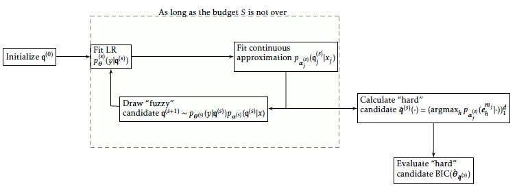
The full algorithm is described schematically in Figure [13].
Numerical experiments
This section is divided into three complementary parts to assess the validity of our proposal, that is called hereafter glmdisc-NN and glmdisc-SEM, designating respectively the approaches developed in Sections 1.4 and 1.5. First, simulated data are used to evaluate its ability to recover the true data generating mechanism. Second, the predictive quality of the new learned representation approach is illustrated on several classical benchmark datasets from the UCI library. Third, we use it on Credit Scoring datasets provided by CACF.
Simulated data: empirical consistency and robustness
Focus is here given on discretization of continuous features (similar experiments could be conducted on categorical ones). Two continuous features \(x_1\) and \(x_2\) are sampled from the uniform distribution on [0, 1] and discretized as exemplified on Figure [14] by using
$$\boldsymbol{q}_1(\cdot)=\boldsymbol{q}_2(\cdot) = ({1}_{]-\infty,1/3]}(\cdot),{1}_{]1/3,2/3]}(\cdot),{1}_{]2/3,\infty[}(\cdot)).$$
Here, we have d = 2 and m1 = m2 = 3 and the cutpoints are cj, 1 = 1/3 and cj, 2 = 2/3 for j = 1, 2. Setting \(\boldsymbol{\theta}=(0,-2,2,0,-2,2,0)\), the target feature y is then sampled from \(p_{\boldsymbol{\theta}}(\cdot | \boldsymbol{q}(\boldsymbol{\mathbf{x}}))\) via the logistic model.
From the glmdisc algorithm, we studied three cases:
First, the quality of the cutoff estimator ĉj, 2 of cj, 2 = 2/3 is assessed when the starting maximum number of intervals per discretized continuous feature is set to its true value m1 = m2 = 3;
Second, we estimated the number of intervals m̂1 of m1 = 3 when the starting maximum number of intervals per discretized continuous feature is set to mmax = 10;
Last, we added a third feature \(x_3\) also drawn uniformly on [0, 1] but uncorrelated to \(y\) and estimated the number m̂3 of discretization intervals selected for \(x_3\). The reason is that a non-predictive feature which is discretized or grouped into a single value is de facto excluded from the model, and this is a positive side effect.
From a statistical point of view, experiment (a) assesses the empirical consistency of the estimation of Cj, h, whereas experiments (b) and (c) focus on the consistency of the estimation of \(m_j\). The results are summarized in Table [2] where 95% confidence intervals (CI (32)) are given, with a varying sample size. Note in particular that the slight underestimation in (b) is a classical consequence of the BIC criterion on small samples.
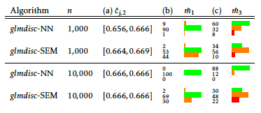
The neural network approach glmdisc-NN seems to outperform the SEM approach on experiments (b) and (c) where the true number of levels \(\boldsymbol{m}\) has to be estimated. This is rather surprising since theoretically, the SEM approach can explore the model space easier than glmdisc-SEM thanks to the additional “disappearing” effect of the drawing procedure (the absorbing state of the MCMC: see Section 1.5.3). This inferior performance is somewhat confirmed with real data in the subsequent sections. A rough guess about this performance drop with an equivalent computational budget S is the “noise” introduced by drawing \(\boldsymbol{\mathfrak{q}}\) rather than maximizing directly the log-likelihood \(\ell_{\boldsymbol{q},\boldsymbol{\alpha}}\) which can be achieved by glmdisc-NN through gradient descent. Therefore, glmdisc-SEM might need way more iterations than glmdisc-NN to converge, especially in a misspecified model setting.
To complement these experiments on simulated data following a well-specified model, a similar study can be done for categorical features: 10 levels are drawn uniformly and 3 groups of levels, which share the same log-odd ratio, are created. The same phenomenon as in Table [2] is witnessed: the empirical distribution of the estimated number of groups of levels is peaked at its true value of 3.
Finally, it was argued in Section 1.3 that by considering all features when quantizing the data, relying on a multivariate approach could yield better results than classical univariate techniques in presence of correlation. This claim is verified in Table [3] where multivariate heteroskedastic Gaussian data is simulated on which the log odd ratio of y depends linearly (misspecified model setting for the quantized logistic regression). The proposed SEM approach yields significantly better results then ChiMerge and MDLP.
[3]
| ChiMerge | MDLP | glmdisc-SEM | |
|---|---|---|---|
| Performance | 50.1 (1.6) | 77.1 (0.9) | 80.6 (0.6) |
Benchmark data
To test further the effectiveness of glmdisc in a predictive setting, we gathered 6 datasets from the UCI library: the Adult dataset (n = 48, 842, d = 14), the Australian dataset (n = 690, d = 14), the Bands dataset (n = 512, d = 39), the Credit-screening dataset (n = 690, d = 15), the German dataset (n = 1, 000, d = 20) and the Heart dataset (n = 270, d = 13). Each of these datasets have mixed (continuous and categorical) features and a binary response to predict. To get more information about these datasets, their respective features, and the predictive task associated with them, readers may refer to the UCI website3.
Now that the proposed approach was shown empirically consistent, i.e. it is able to find the true quantization in a well-specified setting, it is desirable to verify the previous claim that embedding the learning of a good quantization in the predictive task via glmdisc is better than other methods that rely on ad hoc criteria. As we were primarily interested in logistic regression, I will compare the proposed approach to a naïve linear logistic regression (hereafter ALLR), i.e. on non-quantized data, a logistic regression on continuous discretized data using the now standard MDLP algorithm from (9) and categorical grouped data using χ2 tests of independence between each pair of factor levels and the target in the same fashion as the ChiMerge discretization algorithm proposed by (10) (hereafter MDLP/χ2). In this section and the next, Gini indices are reported on a random 30 % test set and CIs are given following a method found in (32). Table [4] shows our approach yields significantly better results on these rather small datasets where the added flexibility of quantization might help the predictive task.
As argued in the preceding section, glmdisc-SEM yields slightly worse results than glmdisc-NN which, additionally to their inherent difference (the S-step of the SEM), might be due to the sensitivity of the SEM to its starting points (a single Markov Chain is run in this section and the next).
| Dataset | ALLR | ad hoc methods | glmdisc-NN | glmdisc-SEM |
| Adult | 81.4 (1.0) | 85.3 (0.9) | 80.4 (1.0) | 81.5 (1.0) |
| Australian | 72.1 (10.4) | 84.1 (7.5) | 92.5 (4.5) | 100 (0) |
| Bands | 48.3 (17.8) | 47.3 (17.6) | 58.5 (12.0) | 58.7 (12.0) |
| Credit | 81.3 (9.6) | 88.7 (6.4) | 92.0 (4.7) | 87.7 (6.4) |
| German | 52.0 (11.3) | 54.6 (11.2) | 69.2 (9.1) | 54.5 (10) |
| Heart | 80.3 (12.1) | 78.7 (13.1) | 86.3 (10.6) | 82.2 (11.2) |
Credit Scoring data
Discretization, grouping and interaction screening are preprocessing steps relatively “manually” performed in the field of Credit Scoring, using χ2 tests for each feature or so-called Weights of Evidence ((33)). This back and forth process takes a lot of time and effort and provides no particular statistical guarantee.
Table [5] shows Gini coefficients of several portfolios for which there are n = 50, 000, n = 30, 000, n = 50, 000, n = 100, 000, n = 235, 000 and n = 7, 500 clients respectively and d = 25, d = 16, d = 15, d = 14, d = 14 and d = 16 features respectively. Approximately half of these features were categorical, with a number of factor levels ranging from 2 to 100. All portfolios come from approximately one year of financed clients. The Automobile dataset is composed of car loans (and thus we have data about the cars, such as the brand, the cost, the motor, etc which generally boosts predictive performance), the Renovation, Mass retail and Electronics datasets are composed of standard loans through partners that respectively sell construction material (to private persons, not companies), retail products (i.e. supermarkets), and electronics goods (smartphones, TVs, etc). The Standard and Revolving datasets are clients coming directly to Sofinco (CACF’s main brand) through the phone or the web.
We compare the rather manual, in-house approach that yields the current performance, the naïve linear logistic regression and ad hoc methods introduced in the previous section and finally our glmdisc proposal. Beside the classification performance, interpretability is maintained and unsurprisingly, the learned representation comes often close to the “manual” approach: for example, the complicated in-house coding of job types is roughly grouped by glmdisc into e.g. “worker”, “technician”, etc. Notice that even if the “naïve” logistic regression reaches some very decent predictive results, its poor interpretability skill (no quantization at all) excludes it from standard use in the company.
Our approach shows approximately similar results than MDLP/χ2, potentially due to the fact that contrary to the two previous experiments with simulated or UCI data, the classes are imbalanced ( < 3% defaulting loans), which would require special treatment while back-propagating the gradients (34). Note however that it is never significantly worse; for the Electronics dataset and as was the case for most UCI datasets, glmdisc is significantly superior, which in the Credit Scoring business might end up saving millions to the financial institution.
Table [6] is somewhat similar but is an earlier work (glmdisc-NN was not implemented at that time): no CI is reported, only continuous features are considered so that pure discretization methods can be compared, namely MDLP and ChiMerge. Three portfolios are used with approx. 10 features and n = 180, 000, n = 30, 000, and n = 100, 000 respectively. The Automobile 2 dataset is again a car loan dataset with information on the cars, the Young clients datasets features only clients less than 30 years old (that are difficult to address in the industry: poor credit history or stability), and the Basel II dataset is a small portion of known clients for which we’d like to provision the expected losses (regulation obligation per the Basel II requirements). The proposed algorithm glmdisc-SEM performs best, but is rather similar to the achieved performance of MDLP. ChiMerge does poorly since its parameter α (the rejection zone of the χ2 tests) is not optimized which is blatant on Portfolio 3 where approx. 2, 000 intervals are created, so that predictions are very “noisy”.
The usefulness of discretization and grouping is clear on Credit Scoring data and although glmdisc does not always perform significantly better than the manual approach, it allows practitioners to focus on other tasks by saving a lot of time, as was already stressed out. As a rule of thumb, a month is generally allocated to data pre-processing for a single data scientist working on a single scorecard. On Google Collaboratory, and relying on Keras ((26)) and Tensorflow ((25)) as a backend, it took less than an hour to perform discretization and grouping for all datasets. As for the glmdisc-SEM method, quantization of datasets of approx. n = 10, 000 observations and approx. d = 10 take about 2 hours on a laptop within a single CPU core. On such a small rig, n = 100, 000 observations and trying to perform interaction screening becomes however prohibitive (approx. 3 days). However, using higher computing power aside, there is still room for improvement, e.g. parallel computing, replacing bottleneck functions with C++ code, etc. Moreover, the ChiMerge and MDLP methods implemented in the R package are not much faster while showing inferior performance and being capable of only discretization on non-missing values.
[5]
| Portfolio | ALLR | Current performance | ad hoc methods | glmdisc-NN | glmdisc-SEM |
| Automobile | 59.3 (3.1) | 55.6 (3.4) | 59.3 (3.0) | 58.9 (2.6) | 57.8 (2.9) |
| Renovation | 52.3 (5.5) | 50.9 (5.6) | 54.0 (5.1) | 56.7 (4.8) | 55.5 (5.2) |
| Standard | 39.7 (3.3) | 37.1 (3.8) | 45.3 (3.1) | 43.8 (3.2) | 36.7 (3.7) |
| Revolving | 62.7 (2.8) | 58.5 (3.2) | 63.2 (2.8) | 62.3 (2.8) | 60.7 (2.8) |
| Mass retail | 52.8 (5.3) | 48.7 (6.0) | 61.4 (4.7) | 61.8 (4.6) | 61.0 (4.7) |
| Electronics | 52.9 (11.9) | 55.8 (10.8) | 56.3 (10.2) | 72.6 (7.4) | 62.0 (9.5) |
[6]
| Portfolio | Current performance | ad hoc methods | glmdisc-NN | glmdisc-SEM |
| Automobile 2 | 57.5 | 16.5 | 58.0 | 58.0 |
| Young clients | 27.0 | 26.7 | 29.2 | 30.0 |
| Basel II | 70.0 | 0 | 71.3 | 71.3 |
Concluding remarks
Handling missing data
For categorical features, handling missing data is straightforward: the level “missing” is simply considered as a separate level, that can eventually be merged in the proposed algorithm with any other level. If it is mnar (e.g. co-borrower information missing because there is none) and such clients are significantly different from other clients in terms of creditworthiness, then such a treatment makes sense. If it is mar and e.g. highly correlated with some of the feature’s levels (for example, the feature “number of children” could be either 0 or missing to mean the borrower has no child), the proposed algorithm is highly likely to group these levels.
For continuous features, the same strategy can be employed: they can be encoded as “missing” and considered a separate level. However, this prevents this level to be merged with another one by having e.g. a level “[0; 200] or missing”.
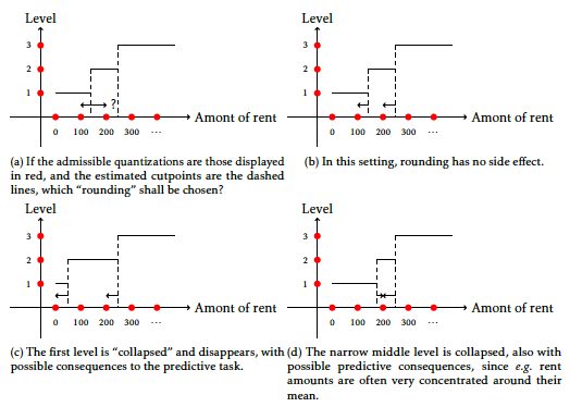
Integrating constraints on the cut-points
Another problem that CACF faces is to have interpretable cutpoints, having discretization intervals of the form [0; 200] and not [0.389; 211.2] which are arguably less interpretable. But it is also highly subjective, and it would require the addition of an hyperparameter, namely the set of admissible discretization and / or the rounding to perform for each feature j such that we did not pursue this problem. For the record, it is interesting to note that a straightforward rounding might not work: in the optimization community, it is well known that integer problems require special algorithmic treatment (dubbed integer programming). As an undergraduate, I applied some of these techniques to financial data in
Wrapping up
Feature quantization (discretization for continuous features, grouping of factor levels for categorical ones) in a supervised multivariate classification setting is a recurring problem in many industrial contexts. This setting was formalized as a highly combinatorial representation learning problem and a new algorithmic approach, named glmdisc, has been proposed as a sensible approximation of a classical statistical information criterion.
The first proposed implementation relies on the use of a neural network of particular architecture and specifically a softmax approximation of each discretized or grouped feature. The second proposed implementation relies on an SEM algorithm and a polytomic multiclass logistic regression approximation in the same flavor as the softmax. These proposals can alternatively be replaced by any other univariate multiclass predictive model, which make them flexible and adaptable to other problems. Prediction of the target feature, given quantized features, was exemplified with logistic regression, although here as well, it can be swapped with any other supervised classification model.
Although both estimation methods are arguably much alike, since they rely on the same continuous approximation, results differed sensibly. Indeed, the SEM approach necessitated a sampling step, whereas the neural network , which has nevertheless the clear advantage of exploring . Additionally, the neural network approach relies on standard deep learning libraries, highly parallelizable and , which can make it way faster than the SEM approach that cannot be parallelized straightforwardly .
The experiments showed that, as was sensed empirically by statisticians in the field of Credit Scoring, discretization and grouping can indeed provide better models than standard logistic regression. This novel approach allows practitioners to have a fully automated and statistically well-grounded tool that achieves better performance than ad hoc industrial practices at the price of decent computing time but much less of the practitioner’s valuable time.
| [1] | David W Hosmer Jr, Stanley Lemeshow, and Rodney X Sturdivant. Applied logistic regression, volume 398. John Wiley & Sons, 2013. [ bib ] |
| [2] | Ying Yang and Geoffrey I Webb. Discretization for naive-bayes learning: managing discretization bias and variance. Machine learning, 74(1):39-74, 2009. [ bib ] |
| [3] | Aleksandra Maj-Kańska, Piotr Pokarowski, Agnieszka Prochenka, et al. Delete or merge regressors for linear model selection. Electronic Journal of Statistics, 9(2):1749-1778, 2015. [ bib ] |
| [4] | Cédric Villani, Yann Bonnet, Charly Berthet, François Levin, Marc Schoenauer, Anne-Charlotte Cornut, and Bertrand Rondepierre. Donner un sens à l'intelligence artificielle: pour une stratégie nationale et européenne. Conseil national du numérique, 2018. [ bib ] |
| [5] | Sergio Ramírez-Gallego, Salvador García, Héctor Mouriño-Talín, David Martínez-Rego, Verónica Bolón-Canedo, Amparo Alonso-Betanzos, José Manuel Benítez, and Francisco Herrera. Data discretization: taxonomy and big data challenge. Wiley Interdisciplinary Reviews: Data Mining and Knowledge Discovery, 6(1):5-21, 2016. [ bib ] |
| [6] | James Dougherty, Ron Kohavi, and Mehran Sahami. Supervised and unsupervised discretization of continuous features. In Machine Learning Proceedings 1995, pages 194-202. Elsevier, 1995. [ bib ] |
| [7] | Huan Liu, Farhad Hussain, Chew Lim Tan, and Manoranjan Dash. Discretization: An enabling technique. Data mining and knowledge discovery, 6(4):393-423, 2002. [ bib ] |
| [8] | Gordon V Kass. An exploratory technique for investigating large quantities of categorical data. Applied statistics, pages 119-127, 1980. [ bib ] |
| [9] | Usama Fayyad and Keki Irani. Multi-interval discretization of continuous-valued attributes for classification learning. In 13th International Joint Conference on Artificial Intelligence, pages 1022–-1029, 1993. [ bib ] |
| [10] | Randy Kerber. Chimerge: Discretization of numeric attributes. In Proceedings of the tenth national conference on Artificial intelligence, pages 123-128. Aaai Press, 1992. [ bib ] |
| [11] | Huan Liu and Rudy Setiono. Chi2: Feature selection and discretization of numeric attributes. In Tools with artificial intelligence, 1995. proceedings., seventh international conference on, pages 388-391. IEEE, 1995. [ bib ] |
| [12] | Ke Wang and Bing Liu. Concurrent discretization of multiple attributes. In Pacific Rim International Conference on Artificial Intelligence, pages 250-259. Springer, 1998. [ bib ] |
| [13] | Francis EH Tay and Lixiang Shen. A modified chi2 algorithm for discretization. IEEE Transactions on Knowledge & Data Engineering, (3):666-670, 2002. [ bib ] |
| [14] | Chao-Ton Su and Jyh-Hwa Hsu. An extended chi2 algorithm for discretization of real value attributes. IEEE transactions on knowledge and data engineering, 17(3):437-441, 2005. [ bib ] |
| [15] | Juliet Popper Shaffer. Multiple hypothesis testing. Annual review of psychology, 46(1):561-584, 1995. [ bib ] |
| [16] | KM Ho and PD Scott. Zeta: a global method for discretization of cotitinuous variables. In Proceedings of the 3rd International Conference on Knowledge Discovery and Data Mining, pages 191-194, 1997. [ bib ] |
| [17] | KM Ho and Paul D Scott. An efficient global discretization method. In Pacific-Asia Conference on Knowledge Discovery and Data Mining, pages 383-384. Springer, 1998. [ bib ] |
| [18] | Hirotugu Akaike. Information theory and an extension of the maximum likelihood principle. In 2nd International Symposium on Information Theory, 1973, pages 267-281. Akademiai Kiado, 1973. [ bib ] |
| [19] | Jiahua Chen and Zehua Chen. Extended bayesian information criteria for model selection with large model spaces. Biometrika, 95(3):759-771, 2008. [ bib ] |
| [20] | Vincent Vandewalle. How to take into account the discrete parameters in the bic criterion? In COMPStat, 2010. [ bib ] |
| [21] | Allou Samé, Faicel Chamroukhi, Gérard Govaert, and Patrice Aknin. Model-based clustering and segmentation of time series with changes in regime. Advances in Data Analysis and Classification, 5(4):301-321, 2011. [ bib ] |
| [22] | Faicel Chamroukhi, Allou Samé, Gérard Govaert, and Patrice Aknin. A regression model with a hidden logistic process for feature extraction from time series. In Neural Networks, 2009. IJCNN 2009. International Joint Conference on, pages 489-496. IEEE, 2009. [ bib ] |
| [23] | Paul Reverdy and Naomi Ehrich Leonard. Parameter estimation in softmax decision-making models with linear objective functions. IEEE Transactions on Automation Science and Engineering, 13(1):54-67, 2016. [ bib ] |
| [24] |
Steven G. Self and Kung-Yee Liang.
Asymptotic properties of maximum likelihood estimators and likelihood
ratio tests under nonstandard conditions.
Journal of the American Statistical Association,
82(398):605-610, 1987.
[ bib |
http ]
Large sample properties of the likelihood function when the true parameter value may be on the boundary of the parameter space are described. Specifically, the asymptotic distribution of maximum likelihood estimators and likelihood ratio statistics are derived. These results generalize the work of Moran (1971), Chant (1974), and Chernoff (1954). Some of Chant's results are shown to be incorrect. The approach used in deriving these results follows from comments made by Moran and Chant. The problem is shown to be asymptotically equivalent to the problem of estimating the restricted mean of a multivariate Gaussian distribution from a sample of size 1. In this representation the Gaussian random variable corresponds to the limit of the normalized score statistic and the estimate of the mean corresponds to the limit of the normalized maximum likelihood estimator. Thus the limiting distribution of the maximum likelihood estimator is the same as the distribution of the projection of the Gaussian random variable onto the region of admissible values for the mean. A variety of examples is provided for which the limiting distributions of likelihood ratio statistics are mixtures of chi-squared distributions. One example is provided with a nuisance parameter on the boundary for which the asymptotic distribution is not a mixture of chi-squared distributions.
|
| [25] | Martín Abadi, Ashish Agarwal, Paul Barham, Eugene Brevdo, Zhifeng Chen, Craig Citro, Greg S. Corrado, Andy Davis, Jeffrey Dean, Matthieu Devin, Sanjay Ghemawat, Ian Goodfellow, Andrew Harp, Geoffrey Irving, Michael Isard, Yangqing Jia, Rafal Jozefowicz, Lukasz Kaiser, Manjunath Kudlur, Josh Levenberg, Dandelion Mané, Rajat Monga, Sherry Moore, Derek Murray, Chris Olah, Mike Schuster, Jonathon Shlens, Benoit Steiner, Ilya Sutskever, Kunal Talwar, Paul Tucker, Vincent Vanhoucke, Vijay Vasudevan, Fernanda Viégas, Oriol Vinyals, Pete Warden, Martin Wattenberg, Martin Wicke, Yuan Yu, and Xiaoqiang Zheng. TensorFlow: Large-scale machine learning on heterogeneous systems, 2015. Software available from tensorflow.org. [ bib | http ] |
| [26] | François Chollet et al. Keras. https://keras.io, 2015. [ bib ] |
| [27] | Léon Bottou. Large-scale machine learning with stochastic gradient descent. In Proceedings of COMPSTAT'2010, pages 177-186. Springer, 2010. [ bib ] |
| [28] | Ann A O'Connell. Logistic regression models for ordinal response variables. Number 146. Sage, 2006. [ bib ] |
| [29] |
Gilles Celeux, Didier Chauveau, and Jean Diebolt.
On Stochastic Versions of the EM Algorithm.
Research Report RR-2514, INRIA, 1995.
[ bib |
http |
.pdf ]
Keywords: MONTE-CARLO EXPERIMENTS ; MIXTURE OF DOSTRIBUTION ; INCOMPLETE DATA MODELS ; STOCHASTIC ALGORITHMS |
| [30] | George Casella and Edward I George. Explaining the gibbs sampler. The American Statistician, 46(3):167-174, 1992. [ bib ] |
| [31] | Peter J Green. Reversible jump markov chain monte carlo computation and bayesian model determination. Biometrika, 82(4):711-732, 1995. [ bib ] |
| [32] | Xu Sun and Weichao Xu. Fast implementation of delong's algorithm for comparing the areas under correlated receiver oerating characteristic curves. IEEE Signal Processing Letters, 21(11):1389-1393, 2014. [ bib ] |
| [33] | Guoping Zeng. A necessary condition for a good binning algorithm in credit scoring. Applied Mathematical Sciences, 8(65):3229-3242, 2014. [ bib ] |
| [34] | Rangachari Anand, Kishan G Mehrotra, Chilukuri K Mohan, and Sanjay Ranka. An improved algorithm for neural network classification of imbalanced training sets. IEEE Transactions on Neural Networks, 4(6):962-969, 1993. [ bib ] |
| [35] | Adrien Ehrhardt. Projet recherche : optimisation non-linéaire - application à la création d'indices boursiers. Master's thesis, École Centrale de Lille, 2014. [ bib ] |
| [36] | Dua Dheeru and Efi Karra Taniskidou. UCI machine learning repository, 2017. [ bib | http ] |