MissImp Test

library(stats)
library(MissImp)
# knitr::opts_chunk$set(eval = FALSE)

Test on the abalone data

In the package, 100 rows of the abalone dataset is stored to test different functions.

load("../data/test_abalone.rda")

abalone_data <- data.frame(test_abalone)
col_num <- c(1:8)
col_dis <- c(8)
col_cat <- c(9)
for (j in col_num) {
  if (j %in% col_dis) {
    suppressWarnings(abalone_data[, j] <- as.integer(abalone_data[, j]))
  }
  else {
    suppressWarnings(abalone_data[, j] <- as.numeric(abalone_data[, j]))
  }
}
for (j in col_cat) {
  abalone_data[, j][abalone_data[, j] == "?"] <- NA
  suppressWarnings(abalone_data[, j] <- as.factor(abalone_data[, j]))
}
abalone_data <- stats::na.omit(abalone_data)
row.names(abalone_data) <- c(1:nrow(abalone_data))
head(abalone_data)

##      V2    V3    V4     V5     V6     V7    V8 V9 V1
## 1 0.455 0.365 0.095 0.5140 0.2245 0.1010 0.150 15  M
## 2 0.350 0.265 0.090 0.2255 0.0995 0.0485 0.070  7  M
## 3 0.530 0.420 0.135 0.6770 0.2565 0.1415 0.210  9  F
## 4 0.440 0.365 0.125 0.5160 0.2155 0.1140 0.155 10  M
## 5 0.330 0.255 0.080 0.2050 0.0895 0.0395 0.055  7  I
## 6 0.425 0.300 0.095 0.3515 0.1410 0.0775 0.120  8  I

After loading and preprocessing the abalone dataset, we can create incomplete datasets with different mechanisms and proportions of missing data. Here for demonstration we chose the "MAR1" missing data mechanism and 20% missing data percentage. (More details about the generation of missing data could be found in vignette "A_Generate_Missingness_and_Tests_MCAR")

X.complete <- abalone_data
mech <- "MAR1"
miss_prop <- 0.3
rs <- generate_miss(X.complete, miss_prop, mechanism = mech)

Then a model could be chosen to impute the incomplete dataset. The parameters shown below need to be chosen wisely.

df <- rs$X.incomp
df_complete <- X.complete
col_cat <- c(9)
col_dis <- c(8)
col_num <- c(1:8)

maxiter_tree <- 10
maxiter_pca <- 200
maxiter_mice <- 10
ncp_pca <- round(ncol(df_complete) / 2)
learn_ncp <- FALSE

num_mi <- 4
n_resample <- 4
n_df <- 5

imp_method <- "MI_Ranger"
resample_method <- "bootstrap"
cat_combine_by <- "onehot"
var_cat <- "wilcox_va"

The initial incomplete dataset, the imputed dataset and the uncertainty for each imputed data are shown below as well as the performance matrices such as MSE(Mean Squared Error) for numerical columns and F1-score for the categorical ones (if the complete dataset is given).

There are two types of MSE that are calculated. The is the normal one that compares the L2 distance between the complete dataset and the imputed one. However, in this case, the columns with higher data values could weight more in MSE than other columns. So, for , before performing the calculation of MSE, the imputed data set and complete dataset are both scaled with Min-Max scale using the parameter from complete dataset.

It is also normal that some lines in are . This comes form the fact that there are too little number of resampled dataset (). If in all those resampled dataset, a certain line shows only once and thus is imputed only once, there is no calculation for the uncertainty of imputation.

head(df)

##      V2    V3    V4     V5     V6     V7    V8 V9   V1
## 1 0.455 0.365 0.095 0.5140 0.2245 0.1010 0.150 15    M
## 2 0.350 0.265 0.090 0.2255 0.0995     NA 0.070  7 <NA>
## 3 0.530 0.420 0.135 0.6770 0.2565 0.1415 0.210  9    F
## 4    NA 0.365 0.125 0.5160 0.2155 0.1140 0.155 10    M
## 5 0.330 0.255 0.080 0.2050 0.0895 0.0395    NA  7    I
## 6 0.425 0.300 0.095 0.3515 0.1410 0.0775 0.120  8    I

head(res$imp)

##          V2    V3    V4     V5     V6         V7         V8 V9 V1
## 1 0.4550000 0.365 0.095 0.5140 0.2245 0.10100000 0.15000000 15  M
## 2 0.3500000 0.265 0.090 0.2255 0.0995 0.04207865 0.07000000  7  I
## 3 0.5300000 0.420 0.135 0.6770 0.2565 0.14150000 0.21000000  9  F
## 4 0.4698935 0.365 0.125 0.5160 0.2155 0.11400000 0.15500000 10  M
## 5 0.3300000 0.255 0.080 0.2050 0.0895 0.03950000 0.06622917  7  I
## 6 0.4250000 0.300 0.095 0.3515 0.1410 0.07750000 0.12000000  8  I

head(res$imp.disj)

##          V2    V3    V4     V5     V6         V7         V8 V9        V1_F
## 1 0.4550000 0.365 0.095 0.5140 0.2245 0.10100000 0.15000000 15 0.000000000
## 2 0.3500000 0.265 0.090 0.2255 0.0995 0.04207865 0.07000000  7 0.003472222
## 3 0.5300000 0.420 0.135 0.6770 0.2565 0.14150000 0.21000000  9 1.000000000
## 4 0.4698935 0.365 0.125 0.5160 0.2155 0.11400000 0.15500000 10 0.000000000
## 5 0.3300000 0.255 0.080 0.2050 0.0895 0.03950000 0.06622917  7 0.000000000
## 6 0.4250000 0.300 0.095 0.3515 0.1410 0.07750000 0.12000000  8 0.000000000
##        V1_I     V1_M
## 1 0.0000000 1.000000
## 2 0.7000868 0.296441
## 3 0.0000000 0.000000
## 4 0.0000000 1.000000
## 5 1.0000000 0.000000
## 6 1.0000000 0.000000

head(res$uncertainty)

##             V2 V3 V4 V5 V6           V7           V8 V9            V1
## 1 0.000000e+00  0  0  0  0 0.000000e+00 0.0000000000  0 -2.220446e-16
## 2 0.000000e+00  0  0  0  0 4.503686e-05 0.0000000000  0  5.000000e-01
## 3 0.000000e+00  0  0  0  0 0.000000e+00 0.0000000000  0 -2.220446e-16
## 4 4.377765e-06  0  0  0  0 0.000000e+00 0.0000000000  0 -2.220446e-16
## 5 0.000000e+00  0  0  0  0 0.000000e+00 0.0002153138  0 -2.220446e-16
## 6 0.000000e+00  0  0  0  0 0.000000e+00 0.0000000000  0 -2.220446e-16

head(res$uncertainty.disj)

##             V2 V3 V4 V5 V6           V7           V8 V9         V1_F      V1_I
## 1 0.000000e+00  0  0  0  0 0.000000e+00 0.0000000000  0 0.000000e+00 0.0000000
## 2 0.000000e+00  0  0  0  0 4.503686e-05 0.0000000000  0 4.822531e-05 0.1044628
## 3 0.000000e+00  0  0  0  0 0.000000e+00 0.0000000000  0 0.000000e+00 0.0000000
## 4 4.377765e-06  0  0  0  0 0.000000e+00 0.0000000000  0 0.000000e+00 0.0000000
## 5 0.000000e+00  0  0  0  0 0.000000e+00 0.0002153138  0 0.000000e+00 0.0000000
## 6 0.000000e+00  0  0  0  0 0.000000e+00 0.0000000000  0 0.000000e+00 0.0000000
##        V1_M
## 1 0.0000000
## 2 0.1062592
## 3 0.0000000
## 4 0.0000000
## 5 0.0000000
## 6 0.0000000

res$MSE

## $list_MSE
## [1] 1.1255460 1.8012099 0.7347307 2.1940199
## 
## $Mean_MSE
## [1] 1.463877
## 
## $Variance_MSE
## [1] 0.4310081
## 
## $list_MSE_scale
## [1] 0.01106567 0.01587142 0.01192461 0.01628618
## 
## $Mean_MSE_scale
## [1] 0.01378697
## 
## $Variance_MSE_scale
## [1] 7.154938e-06

res$F1

## $list_F1
## [1] 0.5333333 0.4705882 0.5000000 0.3333333
## 
## $Mean_F1
## [1] 0.4593137
## 
## $Variance_F1
## [1] 0.007710816

At last, we perform a simple mean imputation as the baseline imputation method. After choosing a certain column (V5 in the example), we can compare the density distribution of the missing values, the imputed values by the method chosen above and the mean imputed values.

res_mean_imp <- df
col_num <- c(1:8)
col_num_name <- colnames(df)[col_num]
for (y in col_num_name) {
  res_mean_imp[[y]][is.na(res_mean_imp[[y]])] <- mean(res_mean_imp[[y]], na.rm = TRUE)
}


ycol <- "V5"
X.miss <- X.complete
X.miss[!is.na(df)] <- NA
dat <- data.frame(
  y = c(X.complete[[ycol]][rs$R.mask[[ycol]]], res$imp[[ycol]][rs$R.mask[[ycol]]], res_mean_imp[[ycol]][rs$R.mask[[ycol]]]),
  lines = rep(c("complete", "imputed", "mean_imputed"), each = sum(rs$R.mask[[ycol]]))
)
ggplot2::ggplot(dat, ggplot2::aes(x = y, fill = lines)) +
  ggplot2::geom_density(alpha = 0.3) +
  ggplot2::labs(x = ycol)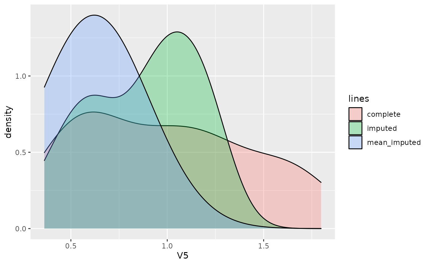

dat <- data.frame(
  y = c(X.miss[[ycol]][rs$R.mask[[ycol]]] - res$imp[[ycol]][rs$R.mask[[ycol]]], X.miss[[ycol]][rs$R.mask[[ycol]]] - res_mean_imp[[ycol]][rs$R.mask[[ycol]]]),
  lines = rep(c("imputed_error", "mean_imputed_error"), each = sum(rs$R.mask[[ycol]]))
)
ggplot2::ggplot(dat, ggplot2::aes(x = y, fill = lines)) +
  ggplot2::geom_density(alpha = 0.3) +
  ggplot2::labs(x = ycol)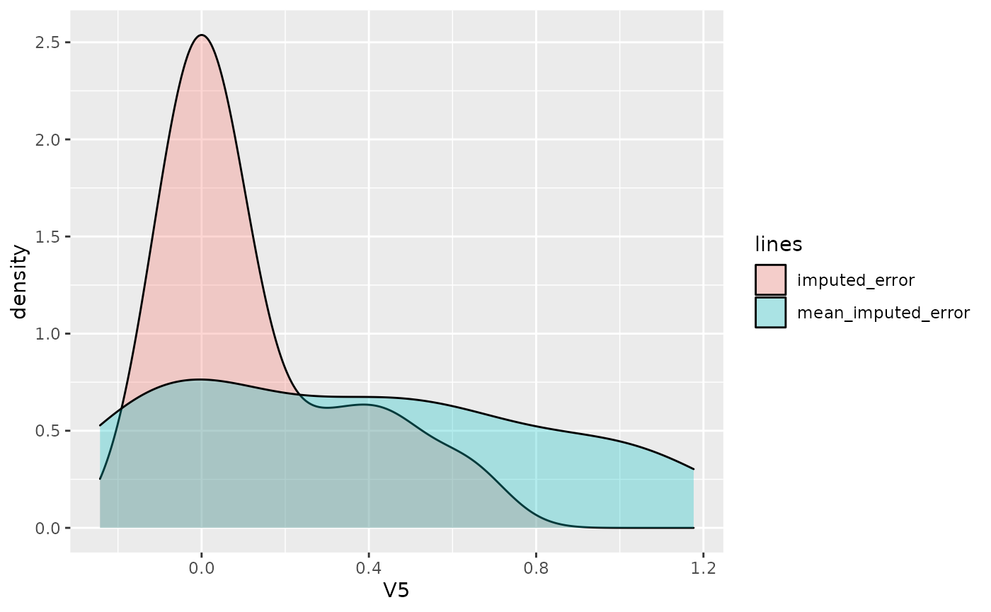

# dat <- data.frame(
#  y = c(X.miss[[ycol]], df[[ycol]]),
#  lines = rep(c("missing", "observed"), each = length(df[[ycol]]))
# )
# ggplot2::ggplot(dat, ggplot2::aes(x = y, fill = lines)) +
#  ggplot2::geom_density(alpha = 0.3) +
#  ggplot2::labs(x = ycol)

Xuwen Liu

2022-03-31

Test on the abalone data